

使用 PyCharm 将 MySQL 数据库中的数据读入 pandas

在数据科学之旅中,您迟早会遇到需要从数据库中获取数据的情况。 然而,从将本地存储的 CSV 文件读入 pandas 到连接和查询数据库,这可能是一项艰巨的任务。 在一系列博文的第一篇中,我们会探讨如何将存储在 MySQL 数据库中的数据读入 pandas,并查看 PyCharm 中使这项任务更简单的一些功能。
查看数据库内容
在本教程中,我们会将一些关于航空公司延误和取消的数据从 MySQL 数据库读取到 pandas DataFrame 中。 这些数据是 Airline Delays from 2003-2016 数据集的一个版本,该数据集由 Priank Ravichandar 提供,以 CC0 1.0 授权。
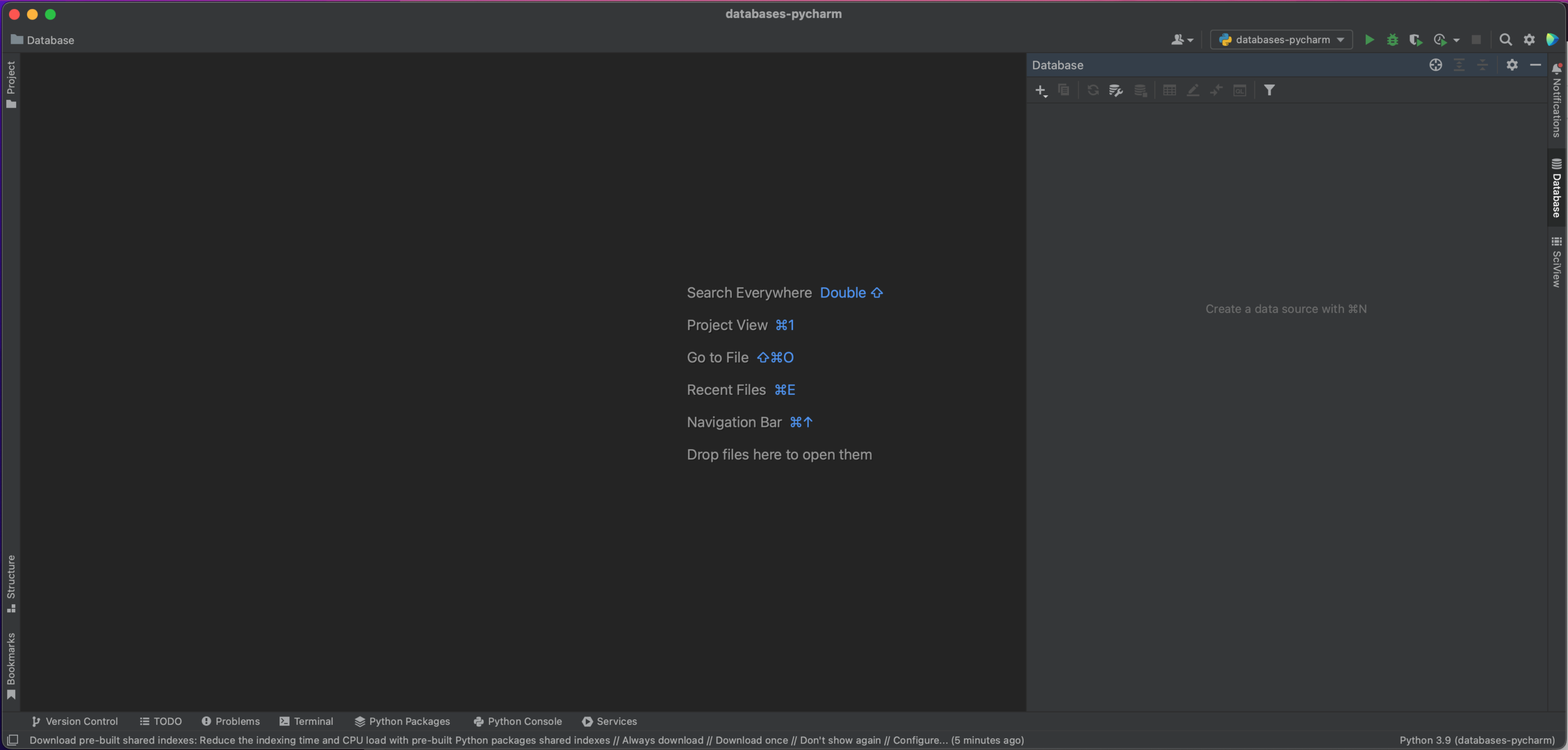
使用数据库可能令人感到困惑的第一件事是无法简要了解可用数据,因为所有表都存储在远程服务器上。 因此,我们要使用的第一个 PyCharm 功能是 Database(数据库)工具窗口,它允许您在进行任何查询之前连接到数据库并对其进行全面内省。
为了连接到我们的 MySQL 数据库,我们首先要导航到 PyCharm 的右侧,然后点击 Database(数据库)工具窗口。
在这个窗口的左上方,您会看到一个加号 (+) 按钮。 点击这个按钮就会出现下面的下拉对话窗口,我们将在其中选择 Data Source | MySQL(数据源 | MySQL)。

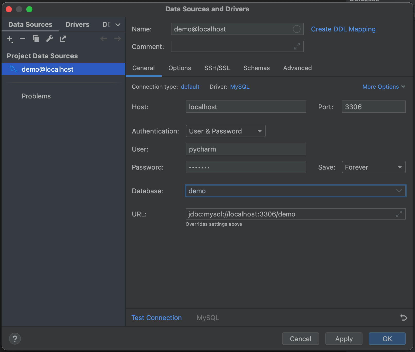
我们现在有一个弹出窗口,它将允许我们连接到我们的 MySQL 数据库。 在这种情况下,我们使用的是本地托管的数据库,因此,我们将 Host(主机)设为“localhost”,将 Port(端口)设为默认的 MySQL 端口“3306”。 我们将使用“用户和密码”作为 Authentication(身份验证)选项,并在 User(用户)和 Password(密码)中输入“pycharm”。 最后,在 Database(数据库)中输入我们的数据库名称“demo”。 当然,要连接到您自己的 MySQL 数据库,您将需要特定主机、数据库名称,以及您的用户名和密码。 请参阅文档了解全部选项。
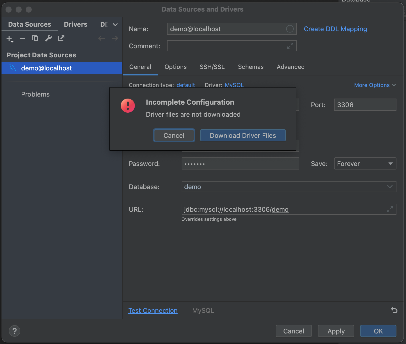
接下来,点击 Test Connection(测试连接)。 PyCharm 提示我们没有安装驱动程序文件。 继续,点击 Download Driver Files(下载驱动程序文件)。 Database(数据库)工具窗口一个非常好的功能是,它会自动为我们找到并安装正确的驱动程序。
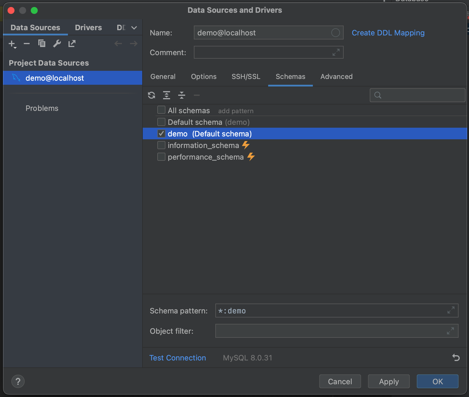
成功! 我们已经连接到我们的数据库。 我们现在可以导航到 Schemas(架构)选项卡,并选择我们想要内省的架构。 在我们的示例数据库中,我们只有一个(“demo”),但在您有非常大的数据库的情况下,可以通过只内省相关数据库来节省时间。
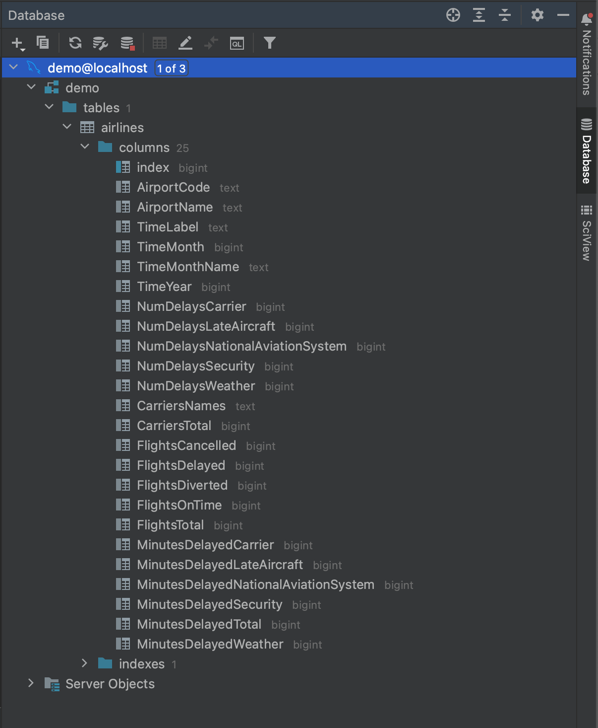
所有这些都完成后,我们就可以连接到我们的数据库了。 点击 OK(确定),然后等待几秒钟。 现在可以看到,我们的整个数据库已被内省,直到表字段级别及其类型。 这使我们在运行查询之前就能对数据库中的内容有一个很好的了解。
使用 MySQL Connector 读入数据
现在,我们已经知道数据库中的内容,可以准备进行查询了。 假设我们想要查看 2016 年至少有 500 次延误的机场。 通过查看内省的 airlines 表中的字段,我们看到我们可以通过以下查询获得这些数据:
SELECT AirportCode,
      SUM(FlightsDelayed) AS TotalDelayed
   FROM airlines
   WHERE TimeYear = 2016
   GROUP BY AirportCode
   HAVING SUM(FlightsDelayed) > 500;
我们使用 Python 运行这个查询的第一种方式是使用一个叫作 MySQL Connector 的软件包,它可以从 PyPI 或 Anaconda 安装。 如果需要关于设置 pip 或 conda 环境或安装依赖项的指导,请参阅链接的文档。 一旦安装完成,我们将打开一个新的 Jupyter Notebook 并导入 MySQL Connector 和 pandas。
import mysql.connector
import pandas as pd
为了从我们的数据库中读取数据,我们需要创建一个连接器。 这是通过 connect 方法完成的,我们向该方法传递访问数据库所需的凭据:host、database 名称、user 和 password。 这些是我们在上一节中使用 Database(数据库)工具窗口访问数据库时使用的相同凭据。
mysql_db_connector = mysql.connector.connect(
   host="localhost",
   database="demo",
   user="pycharm",
   password="pycharm"
)
我们现在需要创建一个游标。 这将用于执行我们对数据库的 SQL 查询,它使用在我们的连接器中存储的凭据来获得访问权限。
mysql_db_cursor = mysql_db_connector.cursor()
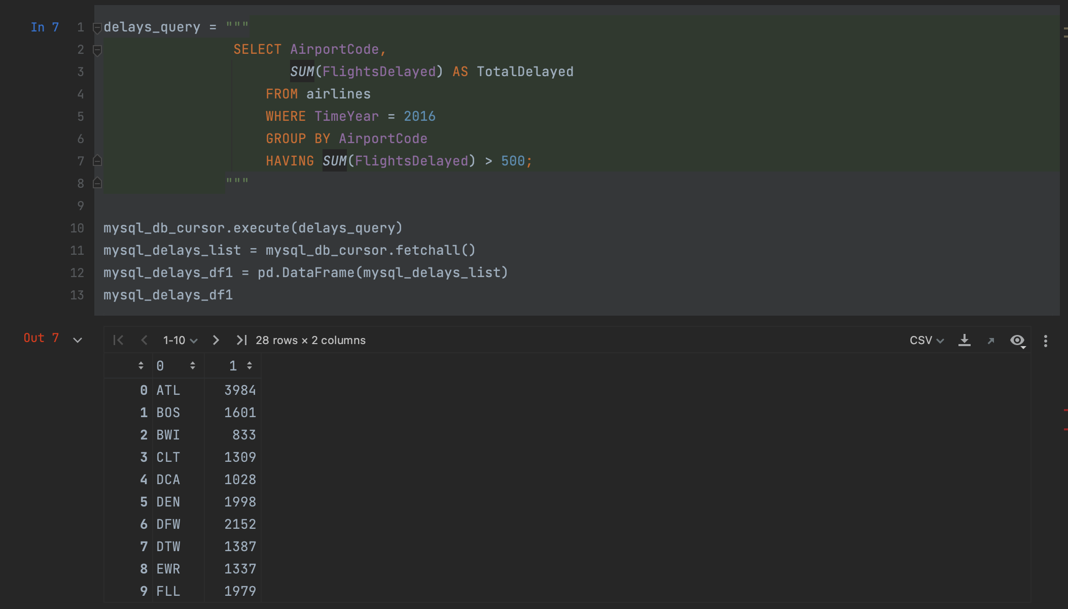
我们现在可以执行查询了。 我们使用游标中的 execute 方法来执行查询,并将查询作为实参传递。
delays_query = """
               SELECT AirportCode,
                      SUM(FlightsDelayed) AS TotalDelayed
                   FROM airlines
                   WHERE TimeYear = 2016
                   GROUP BY AirportCode
                   HAVING SUM(FlightsDelayed) > 500;
              """

mysql_db_cursor.execute(delays_query)
然后,我们使用游标的 fetchall 方法检索结果。
mysql_delays_list = mysql_db_cursor.fetchall()
不过,在这一点上我们有一个问题:fetchall 以列表形式返回数据。 为了将其读入 pandas,我们可以将其传入一个 DataFrame,但是我们会失去列名。如果我们想要创建 DataFrame,则需要手动指定列名。
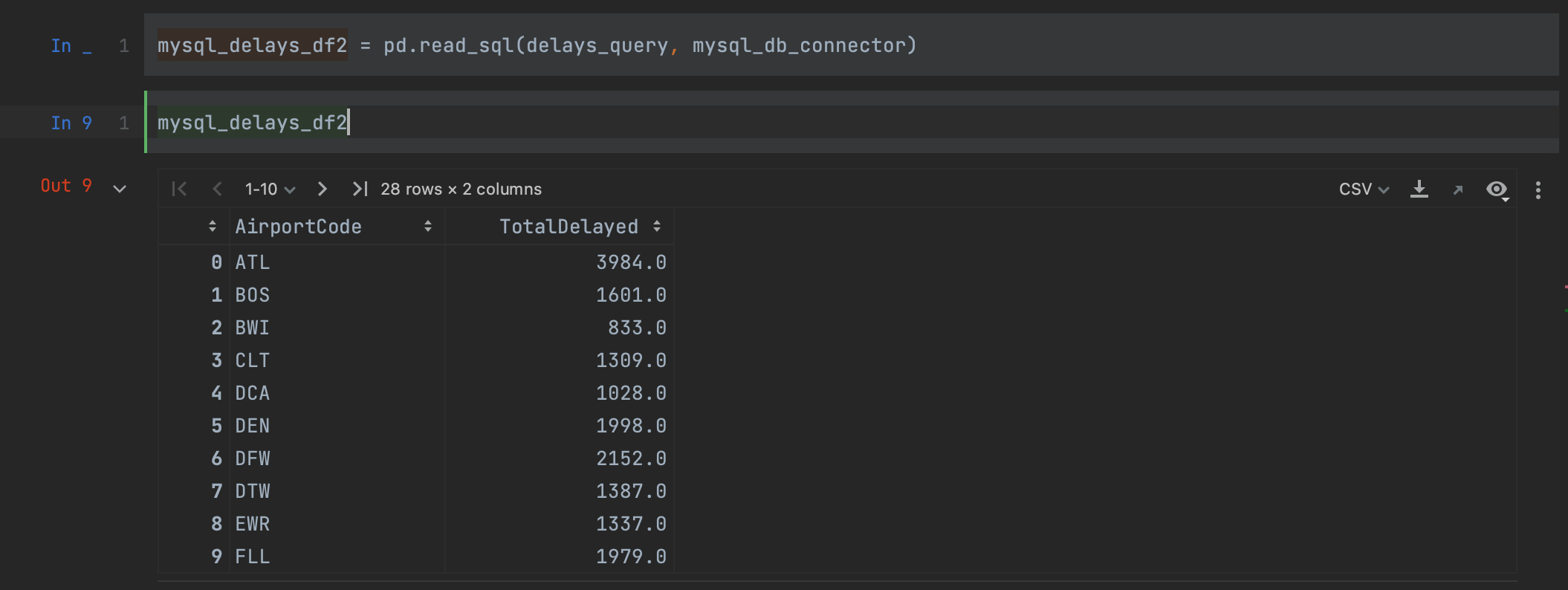
幸好,pandas 提供了一种更好的方式。 我们可以使用 read_sql 方法,一步将我们的查询读入一个 DataFrame,不需要创建游标。
mysql_delays_df2 = pd.read_sql(delays_query, con=mysql_db_connector)
我们只需要将我们的查询和连接器作为实参传递,以便从 MySQL 数据库中读取数据。 查看我们的 DataFrame,我们可以看到我们获得了与上面完全一样的结果,但这次列名被保留了。
您可能已经注意到 PyCharm 有一个不错的功能,这个功能可以将语法高亮显示应用于 SQL 查询,即使查询包含在 Python 字符串中也可以。 稍后在本博文中,我们将介绍 PyCharm 允许您使用 SQL 的另一种方式。
使用 SQLAlchemy 读入数据
使用 MySQL Connector 的另一种方式是使用一个叫作 SQLAlchemy 的软件包。 这个软件包提供了一种一站式方式,可以连接到包括 MySQL 在内的一系列不同的数据库。 使用 SQLAlchemy 的一个好处是,查询不同数据库类型的语法在不同的数据库类型中保持一致。如果您正在使用大量不同的数据库,无需记住一堆不同的命令。
首先,我们需要从 PyPI 或 Anaconda 安装 SQLAlchemy。 然后,我们导入 create_engine 方法,当然还有 pandas。
import pandas as pd
from sqlalchemy import create_engine
我们现在需要创建我们的引擎。 这个引擎允许我们告知 pandas 我们使用的是哪种 SQL 方言(在我们的示例中为 MySQL),并向其提供访问我们的数据库所需的凭据。 这些都以一个字符串的形式传递,即 [dialect]://[user]:[password]@[host]/[database]。 我们来看看这对我们的 MySQL 数据库来说是什么样子:
mysql_engine = create_engine("mysql+mysqlconnector://pycharm:pycharm@localhost/demo")
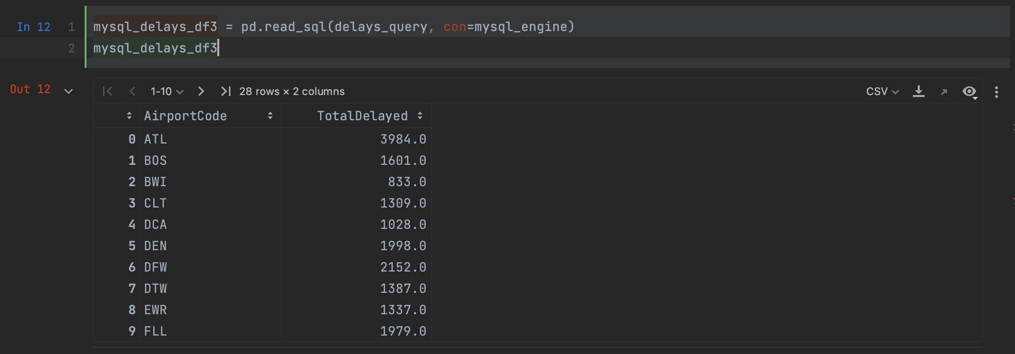
创建引擎后,我们只需要再次使用 read_sql,这次将引擎传递给 con 实参:
mysql_delays_df3 = pd.read_sql(delays_query, con=mysql_engine)
如您所见,我们得到的结果与在 MySQL Connector 中使用 read_sql 时相同。
使用数据库的高级选项
现在,这些连接器方法对于提取我们已经知道自己想要的查询非常好用,但是如果我们想在运行完整查询之前预览我们的数据会是什么样子,或者想知道整个查询会花多长时间,该怎么办? 又到了 PyCharm 大显身手的时候了,它提供了一些使用数据库的高级功能。
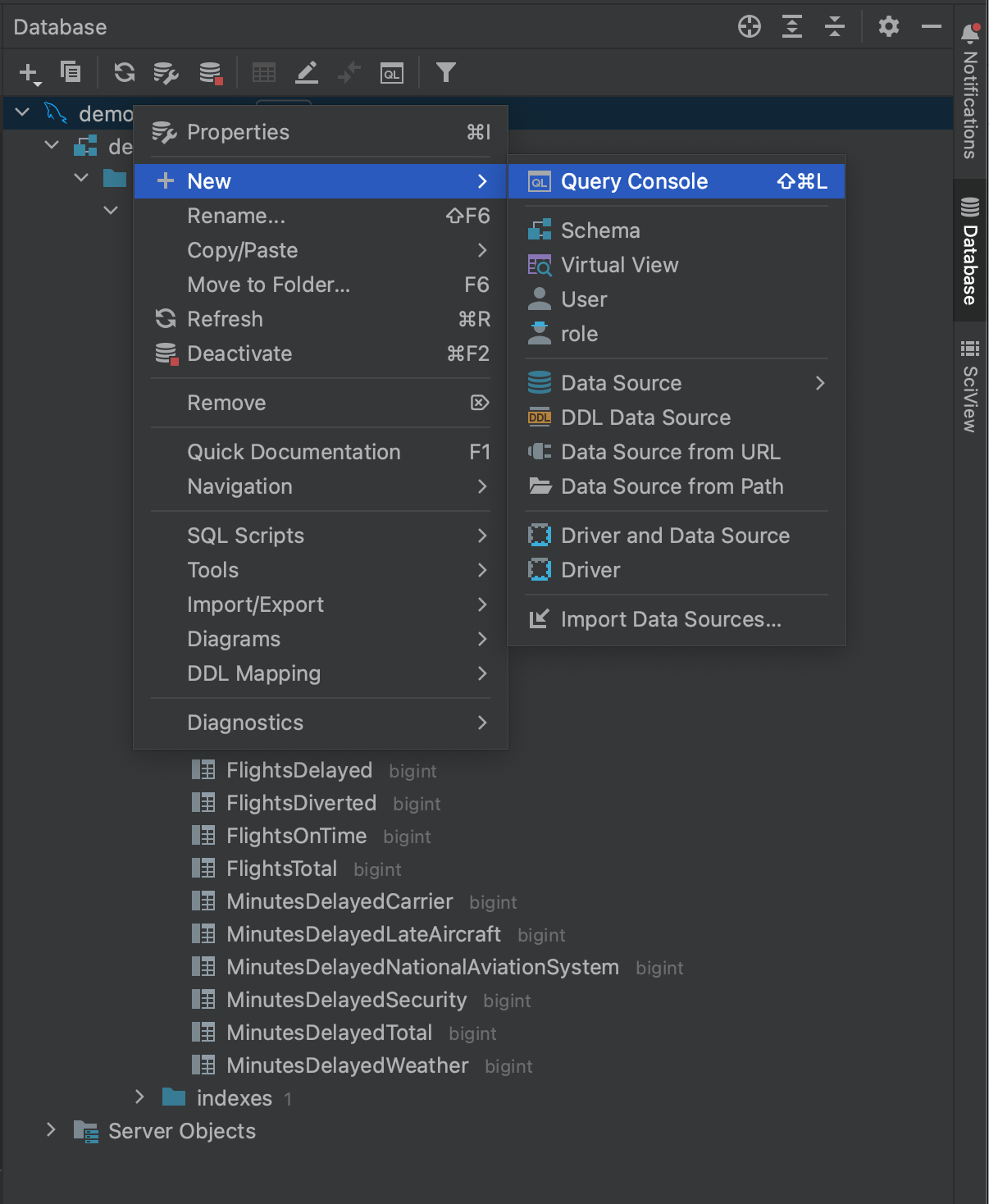
如果我们回到 Database(数据库)工具窗口,右键点击我们的数据库,我们可以看到在 New(新建)下,我们可以创建一个 Query Console(查询控制台)。
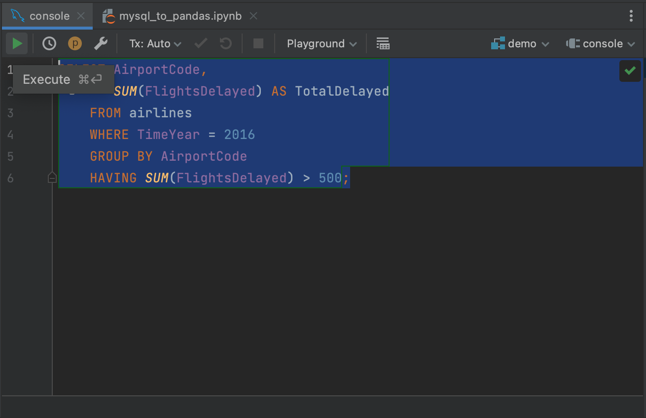
这允许我们打开一个控制台,我们可以用它在原生 SQL 中对数据库进行查询。 控制台窗口包括 SQL 代码补全和内省,这样,您可以更轻松地创建查询,然后再将查询传递给 Python 中的连接器软件包。
高亮显示您的查询,并点击左上角的 Execute(执行)按钮。
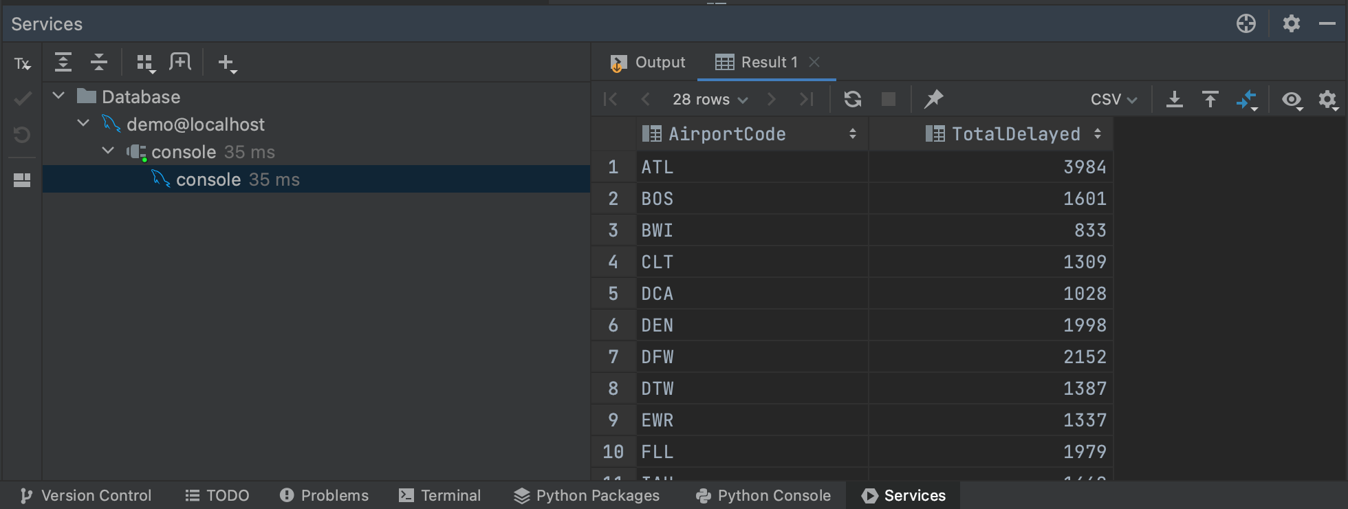
这将在 Services(服务)选项卡中检索我们查询的结果,您可以从这个选项卡检查或导出查询。 对控制台运行查询的一个好处是,最初只从数据库中检索前 500 行,这意味着您可以了解大型查询的结果,而不必提取所有数据。 您可以调整检索的行数:转到 Settings/Preferences | Tools | Database | Data Editor and Viewer(设置/偏好设置 | 工具 | 数据库 | 数据编辑和查看器),并更改 Limit page size to:(将页面大小限制为:)下的值。
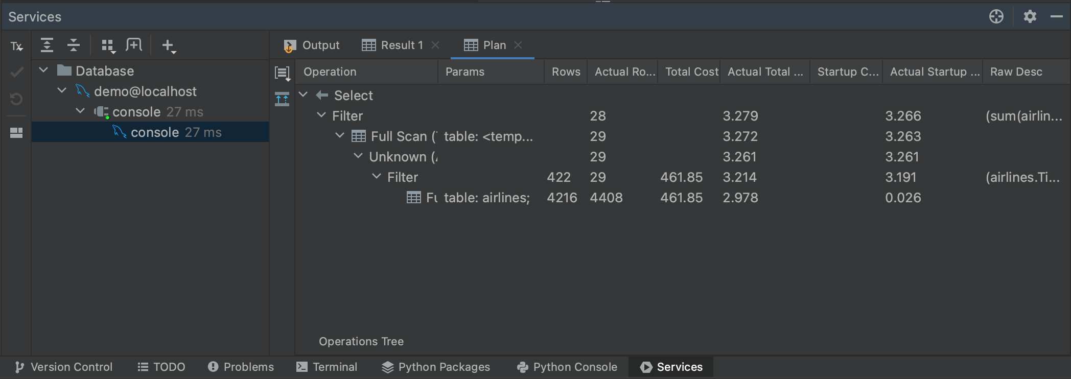
说到大型查询,我们也可以通过生成一个执行计划来了解我们的查询将需要多长时间。 如果我们再次高亮显示我们的查询,然后点击右键,我们可以从菜单中选择 Explain Plan | Explain Analyse。 这将为我们的查询生成一个执行计划,显示查询计划器为检索结果所采取的每一个步骤。 执行计划是它们自己的主题,我们并不需要了解我们的计划所告诉我们的一切。 与我们的目的最相关的是 Actual Total Time(实际总时间)列,在这里我们可以看到在每个步骤中返回所有行需要多长时间。 这让我们能够对整个查询时间有一个很好的估计,以及预判我们查询的任何部分是否可能特别耗时。
您也可以通过点击 Plan(计划)面板左侧的 Show Visualization(显示可视化)按钮来可视化执行。
这将弹出一个流程图,让您更轻松浏览查询计划器正在进行的步骤。
将数据从 MySQL 数据库中读入 pandas DataFrames 非常简单。PyCharm 提供了很多强大的工具来让使用 MySQL 数据库变得更简单。 在下一篇博文中,我们将了解如何使用 PyCharm 将数据从另一种流行的数据库类型 – PostgreSQL 数据库 – 读入 pandas。
本博文英文原作者:

Subscribe to PyCharm Blog updates

Discover more


Using PyCharm to Read Data From a MySQL DataBase Into pandas

Sooner or later in your data science journey, you’ll hit a point where you need to get data from a database. However, making the leap from reading a locally-stored CSV file into pandas to connecting to and querying databases can be a daunting task. In the first of a series of blog posts, we’ll explore how to read data stored in a MySQL database into pandas, and look at some nice PyCharm features that make this task easier.
Viewing the database contents
In this tutorial, we’re going to read some data about airline delays and cancellations from a MySQL database into a pandas DataFrame. This data is a version of the “Airline Delays from 2003-2016” dataset by Priank Ravichandar licensed under CC0 1.0.
One of the first things that can be frustrating about working with databases is not having an overview of the available data, as all of the tables are stored on a remote server. Therefore, the first PyCharm feature we’re going to use is the Database tool window, which allows you to connect to and fully introspect a database before doing any queries.
To connect to our MySQL database, we’re first going to navigate over to the right-hand side of PyCharm and click the Database tool window.
On the top left of this window, you’ll see a plus button. Clicking on this gives us the following dropdown dialog window, from which we’ll select Data Source | MySQL.
We now have a popup window which will allow us to connect to our MySQL database. In this case, we’re using a locally hosted database, so we leave Host as “localhost” and Port as the default MySQL port of “3306”. We’ll use the “User & Password” Authentication option, and enter “pycharm” for both the User and Password. Finally, we enter our Database name of “demo”. Of course, in order to connect to your own MySQL database you’ll need the specific host, database name, and your username and password. See the documentation for the full set of options.
Next, click Test Connection. PyCharm lets us know that we don’t have the driver files installed. Go ahead and click Download Driver Files. One of the very nice features of the Database tool window is that it automatically finds and installs the correct drivers for us.
Success! We’ve connected to our database. We can now navigate to the Schemas tab and select which schemas we want to introspect. In our example database we only have one (“demo”), but in cases where you have very large databases, you can save yourself time by only introspecting relevant ones.
With all of that done, we’re ready to connect to our database. Click OK, and wait a few seconds. You can now see that our entire database has been introspected, down to the level of table fields and their types. This gives us a great overview of what is in the database before running a single query.
Reading in the data using MySQL Connector
Now that we know what is in our database, we are ready to put together a query. Let’s say we want to see the airports that had at least 500 delays in 2016. From looking at the fields in the introspected airlines table, we see that we can get that data with the following query:
SELECT AirportCode,
      SUM(FlightsDelayed) AS TotalDelayed
   FROM airlines
   WHERE TimeYear = 2016
   GROUP BY AirportCode
   HAVING SUM(FlightsDelayed) > 500;
The first way we can run this query using Python is using a package called MySQL Connector, which can be installed from either PyPI or Anaconda. See the linked documentation if you need guidance on setting up pip or conda environments or installing dependencies. Once installation is finished, we’ll open a new Jupyter notebook and import both MySQL Connector and pandas.
import mysql.connector
import pandas as pd
In order to read data from our database, we need to create a connector. This is done using the connect method, to which we pass the credentials needed to access the database: the host, the database name, the user, and the password. These are the same credentials we used to access the database using the Database tool window in the previous section.
mysql_db_connector = mysql.connector.connect(
   host="localhost",
   database="demo",
   user="pycharm",
   password="pycharm"
)
We now need to create a cursor. This will be used to execute our SQL queries against the database, and it uses the credentials sorted in our connector to get access.
mysql_db_cursor = mysql_db_connector.cursor()
We’re now ready to execute our query. We do this using the execute method from our cursor and passing the query as the argument.
delays_query = """
               SELECT AirportCode,
                      SUM(FlightsDelayed) AS TotalDelayed
                   FROM airlines
                   WHERE TimeYear = 2016
                   GROUP BY AirportCode
                   HAVING SUM(FlightsDelayed) > 500;
              """

mysql_db_cursor.execute(delays_query)
We then retrieve the result using the cursor’s fetchall method.
mysql_delays_list = mysql_db_cursor.fetchall()
However, we have a problem at this point: fetchall returns the data as a list. To get it into pandas, we can pass it into a DataFrame, but we’ll lose our column names and will need to manually specify them when we want to create the DataFrame.
Luckily, pandas offers a better way. Rather than creating a cursor, we can read our query into a DataFrame in one step, using the read_sql method.
mysql_delays_df2 = pd.read_sql(delays_query, con=mysql_db_connector)
We simply need to pass our query and connector as arguments in order to read the data from the MySQL database. Looking at our dataframe, we can see that we have the exact same results as above, but this time our column names have been preserved.
A nice feature you might have noticed is that PyCharm applies syntax highlighting to the SQL query, even when it’s contained inside a Python string. We’ll cover another way that PyCharm allows you to work with SQL later in this blog post.
Reading in the data using SQLAlchemy
An alternative to using MySQL Connector is using a package called SQLAlchemy. This package offers a one-stop method for connecting to a range of different databases, including MySQL. One of the nice things about using SQLAlchemy is that the syntax for querying different database types remains consistent across database types, saving you from remembering a bunch of different commands if you’re working with a lot of different databases.
To get started, we need to install SQLAlchemy either from PyPI or Anaconda. We then import the create_engine method, and of course, pandas.
import pandas as pd
from sqlalchemy import create_engine
We now need to create our engine. The engine allows us to tell pandas which SQL dialect we’re using (in our case, MySQL) and provide it with the credentials it needs to access our database. This is all passed as one string, in the form of [dialect]://[user]:[password]@[host]/[database]. Let’s see what this looks like for our MySQL database:
mysql_engine = create_engine("mysql+mysqlconnector://pycharm:pycharm@localhost/demo")
With this created, we simply need to use read_sql again, this time passing the engine to the con argument:
mysql_delays_df3 = pd.read_sql(delays_query, con=mysql_engine)
As you can see, we get the same result as when using read_sql with MySQL Connector.
Advanced options for working with databases
Now these connector methods are very nice for extracting a query that we already know we want, but what if we want to get a preview of what our data will look like before running the full query, or an idea of how long the whole query will take? PyCharm is here again with some advanced features for working with databases.
If we navigate back over to the Database tool window and right-click on our database, we can see that under New we have the option to create a Query Console.
This allows us to open a console which we can use to query against the database in native SQL. The console window includes SQL code completion and introspection, giving you an easier way to create your queries prior to passing them to the connector packages in Python.
Highlight your query and click the Execute button in the top left corner.
This will retrieve the results of our query in the Services tab, where it can be inspected or exported. One nice thing about running queries against the console is that only the first 500 rows are initially retrieved from the database, meaning you can get a sense of the results of larger queries without committing to pulling all of the data. You can adjust the number of rows retrieved by going to Settings/Preferences | Tools | Database | Data Editor and Viewer and changing the value under Limit page size to:.
Speaking of large queries, we can also get a sense of how long our query will take by generating an execution plan. If we highlight our query again and then right-click, we can select Explain Plan | Explain Analyse from the menu. This will generate an execution plan for our query, showing each step that the query planner is taking to retrieve our results. Execution plans are their own topic, and we don’t really need to understand everything our plan is telling us. Most relevant for our purposes is the Actual Total Time column, where we can see how long it will take to return all of the rows at each step. This gives us a good estimate of the overall query time, as well as whether any parts of our query are likely to be particularly time consuming.
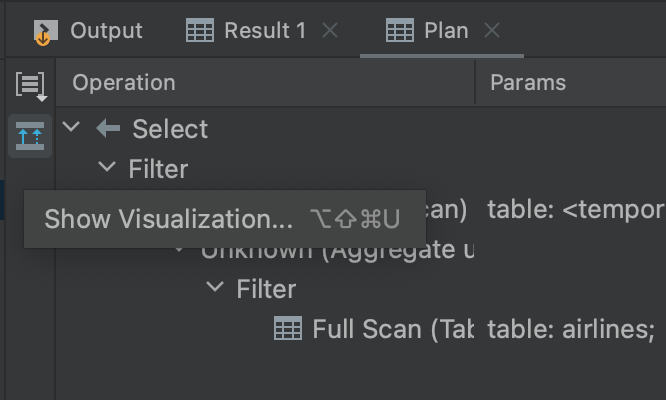
You can also visualize the execution by clicking on the Show Visualization button to the left of the Plan panel.
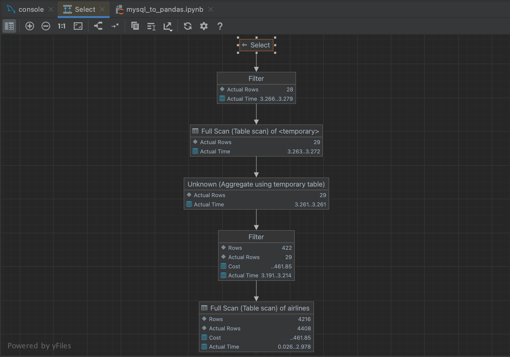
This will bring up a flowchart that makes it a bit easier to navigate through the steps that the query planner is taking.
Getting data from MySQL databases into pandas DataFrames is straightforward, and PyCharm has a number of powerful tools to make working with MySQL databases easier. In the next blog post, we’ll look at how to use PyCharm to read data into pandas from another popular database type, PostgreSQL databases.
Subscribe to PyCharm Blog updates