Best Object Detection Models for Machine Learning in 2026

Object detection powers transformative applications, from autonomous vehicles navigating city streets and security systems identifying threats in real time to retail analytics tracking inventory and medical imaging detecting tumors. But choosing the right model for your computer vision project can be challenging, especially with dozens of architectures claiming superiority across different metrics.
In this guide, we’ll examine the top object detection models available in 2026, comparing their architectures, performance characteristics, and ideal use cases to help you determine which models are best suited to your applications.
Whether you’re building real-time video analytics, high-precision inspection systems, or resource-constrained edge applications, you’ll find clear guidance on which model best fits your requirements.
What is object detection?
Object detection aims to identify and localize multiple objects within images or video frames. Unlike image classification, which only classifies the broad identity of an image, object detection identifies the objects in an image/video frame and their exact positions within it.
In a nutshell, object detection solves two interdependent problems:
- Localizing (detecting) the objects on the image, by drawing the bounding boxes for the objects on the image (it is possible that there are zero objects!). A bounding box is usually defined as a tuple (x, y, h, w), where x and y are the top-left coordinates of the bounding box rectangle, and h and w are the height and width of the bounding box, respectively.
- Classifying the identities of these images (like a person, car, or dog).
This dual capability makes object detection more complex than classification alone, requiring models that can handle multiple objects of different sizes appearing anywhere in an image.
As with classification tasks, a simple accuracy metric is not sufficient to assess model performance. We need metrics of two types. Firstly, performance metrics that gauge the trade-off between incorrectly detecting objects (false positives) and not detecting objects at all in the image when they were present (false negatives). Secondly, we also need metrics to assess how long it will take our model to perform the task in question: We will call these compute efficiency metrics. Usually, the new architectures for object detection are benchmarked on the validation partition of the COCO dataset and run on T4 NVIDIA GPU hardware.
Here are the standard metrics used in the object detection community:
- Basic building block of performance metric: Intersection over union (IoU) is the foundational geometric measure used to decide whether a predicted bounding box is correct. It is calculated as the area of overlap between the predicted box and the ground-truth box, divided by the area of their union – producing a score between 0 (no overlap) and 1 (perfect match). A detection is counted as a true positive only if its IoU with the nearest ground-truth box exceeds a chosen threshold (e.g. 0.5). A low IoU threshold is lenient about box placement; a high one demands tight localization.
- Performance metric: Mean average precision (mAP), which evaluates detection accuracy by measuring how well predicted boxes overlap with ground truth annotations across different confidence thresholds. The most commonly cited variant, mAP@[50:95] (also written AP50:95), averages precision over IoU thresholds from 0.50 to 0.95 in steps of 0.05, which is a stringent measure that penalizes imprecise localization as much as missed detections.
- mAP50 vs. mAP50:95: mAP50 measures detection at IoU ≥ 0.5 and scores appear higher, favoring faster models. mAP50:95 averages across IoU thresholds 0.5–0.95 – the stricter, preferred metric. For precision-critical applications (robotics, medical), it is common to optimize for mAP50:95.
- Compute efficiency metric: Frames per second (FPS), which measures inference speed, determining whether a model can process video in real-time. For standard videos, real-time is defined as >= 30 FPS (Google or original YOLO paper) or latency <= 33.3ms (1/FPS * 1000). Naturally, for such applications as self-driving cars or robotics, there are higher requirements on the FPS rate, going up as high as 60–100+ FPS.
- Compute efficiency metric: Parameter count is a quality of the model that influences its performance. There is a trade-off between the model’s accuracy and its parameter count. That’s why models are provided in different sizes of the same architecture (S, M, L, XL, etc.) to cater to various scenarios of this trade-off. This is similar to the concept of parameter count in LLMs.
There are a few popular choices of datasets to evaluate the performance of object detection models. As mentioned above, the standard choice for benchmarking object detection is the COCO dataset, containing 80 object categories across 330,000 images. Naturally, there are a lot of other datasets, specialized for certain domains, such as self-driving cars, or certain scenarios, such as the detection of objects in cluttered environments. What is important to remember is that the values of object detection metrics, IoU, and mAP depend on the dataset they were evaluated on, so mAP@[50:95]=60.1 on the COCO dataset may not be directly transferable to your custom dataset. These metrics should always be re-evaluated on your dataset to define the baseline performance of the models on it.
Object detection algorithms and architecture families
Object detection models fall into two different processing flows and two different architectural families.
Architectures
CNN-based
Examples: Faster R-CNN, Mask R-CNN, Cascade R-CNN, YOLO
CNN-based detectors rely on convolutional layers to extract local features hierarchically across the image, traditionally using predefined anchor boxes as spatial priors for localizing objects. Spatial priors are predefined assumptions about where and what size objects are likely to appear in an image, giving the model a starting point for detection rather than searching randomly.
Transformer-based
Examples: RF-DETR, RT-DETR, D-FINE
Transformer-based detectors, inspired by advances in natural language processing, instead apply global self-attention mechanisms that allow the model to reason about relationships across the entire image simultaneously.
Specifically, transformer-based detectors use learned object queries and global self-attention, where each query is trained to correspond to at most one object, unlike CNN-based detectors, which build spatial understanding locally through convolutional layers with limited receptive fields.
However, in modern architectures, there exists a fusion of the two architectures: a CNN network can use self-attention modules in its architecture, such as YOLOv12 or YOLOv13, leading to cross-architectural designs.
Processing flows
Two-stage detectors
Examples: Faster R-CNN, Mask R-CNN, Cascade R-CNN
The network makes two sequential passes, each with a distinct job:
- Stage 1: Region Proposal:
- Scans the image and proposes ~1000–2000 candidate regions (RoIs) that might contain objects.
- Doesn’t care about class yet, just the fact that “something interesting is here”.
- This is the region proposal network (RPN) in classic detectors
- Stage 2: RoI classification and refinement:
- Takes only the proposed regions from Stage 1.
- Crops/pools features for each region.
- Predicts the exact class and refined box coordinates for each proposal.
Single-stage detectors
Examples: YOLO series, SSD, RetinaNet, DETR
The network directly predicts class labels and bounding boxes from feature maps. It does everything in one forward pass. Usually, the following happens:
- A dense grid of anchor boxes (or points) is placed over the image.
- For each anchor, the network simultaneously predicts:
- Whether there is an object there (objectness/class score).
- How the box should be adjusted (box regression offsets).
- In older versions of single-stage detectors, one needed to filter overlapping bounding boxes at the end; it was done using the non-maximum suppression (NMS) algorithm. From YOLOv10 on, using NMS is a redundant step.
Furthermore, modern single-stage detectors have moved away from anchor-based designs entirely, predicting box coordinates directly from grid points and pixels, eliminating the need for dataset-specific anchor tuning altogether.
Historically, two-stage detectors offered better accuracy at the cost of speed, but modern single-stage detectors have largely closed this gap, achieving comparable or superior results while remaining significantly faster. Thus, we will focus on single-stage detectors only when evaluating the state-of-the-art models for practical applications.
Top object detection models in 2026
Two-stage pipelines (Faster R-CNN, Mask R-CNN) are no longer competitive. The current frontier is defined by single-stage NMS-free transformer architectures and models of the YOLO family. Each model below excels in a specific deployment scenario.
RF-DETR (by Roboflow) – Highest Accuracy
Real-Time Detection Transformer · ICLR 2026
| Metric | Value |
|---|---|
| mAP50:95 (N) | 48.4 |
| mAP50:95 (M) | 54.7 |
| Latency (N) | 2.3 ms |
| Latency (M) | 4.4 ms |
| mAP50:95 (2XL) | 60.1 (COCO record) |
| Latency (2XL) | 21.8 ms |
The strongest real-time model available. RF-DETR uses DINOv2 to extract deeply rich, globally-aware feature representations of the input image, then uses deformable cross-attention in the detection head to efficiently query those features and predict bounding boxes without needing anchor boxes or NMS post-processing. The result is a model that’s simultaneously more accurate on complex scenes and faster at inference than the naive combination of those components would suggest. RF-DETR is the first real-time detector to break 60 mAP on MS COCO. Designed from the ground up for fine-tuning, DINOv2 pre-training on internet-scale data gives it unmatched domain adaptability across aerial imagery, medical scans, industrial inspection, and more. It comes in four sizes: Nano, Small, Medium, Large (plus XL/2XL under a PML license).
Strengths:
- Highest mAP of any real-time model.
- Exceptional domain transfer (fine-tunes fast).
- Best on occluded and complex scenes.
- Supports detection + segmentation in a single API.
- Apache 2.0, fully commercial-friendly.
Limitations:
- Heavier than YOLO on edge/mobile.
- XL/2XL models require a PML license.
- Higher GPU memory vs. YOLO variants.
License: Apache 2.0 (N/S/M/L) · PML 1.0 (XL/2XL)
Repository: https://github.com/roboflow/rf-detr
YOLO12 (Tsinghua University) – Research / Benchmark
Attention-centric YOLO · NeurIPS 2025
| Metric | Value |
|---|---|
| mAP50:95 (N) | 40.4 |
| mAP50:95 (M) | 52.5 |
| Latency (N) | 1.60 ms |
| Latency (M) | 4.27 ms |
| License | AGPL-3.0 |
YOLO12 is the first YOLO model to place attention mechanisms at the core rather than CNNs, matching CNN-based inference speeds while gaining the global context benefits of self-attention. Key innovations: Area attention (A²) divides feature maps into regions to reduce the quadratic cost of full self-attention; Residual ELAN (R-ELAN) stabilizes training of large attention blocks; FlashAttention reduces memory bottlenecks. It is deployable on NVIDIA Jetson, NVIDIA GPUs, and macOS.
A note on implementations. YOLO12 exists in two separate codebases, and the distinction matters in practice. The original authors (Tsinghua/University at Buffalo) actively maintain their own repository at sunsmarterjie/yolov12. In June 2025, they explicitly warned against using Ultralytics’ integration, stating it “is inefficient, requires more memory, and has unstable training” – issues they have fixed in their own repo. The training instability and memory criticisms often cited against YOLO12 are therefore criticisms of the Ultralytics port, not the model itself. Ultralytics’ recommendation to prefer YOLO26 over YOLO12 should be read with this context in mind: The comparison is partly against their own suboptimal implementation.
If you use YOLO12, install from the original repository rather than via pip install ultralytics.
Strengths:
- Strong accuracy at the nano scale (beats YOLO11-N by 0.9% mAP).
- Long-range context via attention mechanisms: It can take into account the entire image when detecting an object, rather than a local pixel neighborhood, as in pure CNN architectures.
- Jetson-, Android-, and macOS-deployable.
- Original repo fixes memory and training stability issues present in the Ultralytics port.
- Actively maintained by original authors with ongoing updates (turbo variant, segmentation, and classification).
Limitations:
- If using Ultralytics implementation:
- AGPL-3.0 commercial use requires an enterprise license.
- Training instability and high memory on large models.
- If using an open-source implementation:
- AGPL-3.0 commercial use requires an enterprise license.
- Claims to have stable training and inference in comparison with Ulitralytics implementation.
- Requires installing from the original repo to avoid Ultralytics port issues, resulting in slightly more setup friction.
- Smaller ecosystem and community support than Ultralytics-native models.
License: AGPL-3.0 (open-source) · Enterprise license via Ultralytics for commercial use
Open-source repository: https://github.com/sunsmarterjie/yolov12
Ultralytics repository: https://github.com/ultralytics/ultralytics
YOLO26 (Ultralytics) – Best for edge / production
Edge-first unified YOLO · September 2025
| Metric | Value |
|---|---|
| mAP50:95 range | 40.9–57.5 |
| Latency range | 1.7–11.8 ms |
| CPU gain vs. YOLO11 (nano) | +43% |
| Unified tasks | 5 |
Ultralytics’ flagship for 2025–2026. YOLO26 shifts focus from accuracy maximization toward deployment-oriented simplification: It removes NMS and distribution focal loss (DFL) for end-to-end inference, introduces the MuSGD optimizer for stable convergence, and adds progressive loss balancing (ProgLoss), which makes sure that the model doesn’t over-optimize one objective at the expense of others, and small-target-aware label assignment (STAL), which ensures extra attention to small objects. Five tasks are solved by this one YOLO26: detection, segmentation, pose estimation, oriented bounding boxes detection, and open-vocabulary detection and segmentation. It is explicitly designed for NVIDIA Jetson Orin/Xavier, Qualcomm Snapdragon AI, and ARM CPUs. Supports INT8 and FP16 quantization, plus ONNX, TensorRT, CoreML, and TFLite export.
Strengths:
- Best edge and mobile performance (Jetson Orin and Snapdragon).
- NMS-free leads to lower latency.
- 43% faster CPU inference than YOLO11(N) at comparable accuracy, ideal for devices without a GPU.
- Five tasks in one architecture.
- Stable INT8/FP16 quantization.
Limitations:
- AGPL-3.0: commercial use requires an enterprise license.
- Lower peak accuracy than RF-DETR XL.
License: AGPL-3.0 (open-source) · Enterprise license via Ultralytics for commercial/industrial use.
Repository: https://github.com/ultralytics/ultralytics
Benchmark comparison
To give a comparison between the models, here are the exact benchmark values. All scores on MS COCO val2017. Latency was measured on an NVIDIA T4 GPU.
| Model | mAP50 | mAP50:95 | Latency | Params | Edge-ready | License |
|---|---|---|---|---|---|---|
| RF-DETR-N | 67.6 | 48.4 | 2.3 ms | 30.5 M | Server GPU | Apache 2.0 |
| RF-DETR-M | 73.6 | 54.7 | 4.4 ms | 33.7 M | Server GPU | Apache 2.0 |
| RF-DETR-2XL | 78.5 | 60.1 | 17.2 ms | 126.9 M | Server GPU | PML 1.0 |
| YOLO12-N | 56.7 | 40.4 | 1.6 ms | 2.5 M | ARM / Mobile / Jetson | AGPL-3.0 |
| YOLO12-L | 70.7 | 53.8 | 5.83 ms | 26.5 M | Jetson / TensorRT | AGPL-3.0 |
| YOLO26-N | — | 40.1 | 1.7 ms | 2.4 M | ARM / Mobile / Jetson | AGPL-3.0 |
| YOLO26-X | — | 56.9 | 11.8 ms | 55.7 M | Jetson / TensorRT | AGPL-3.0 |
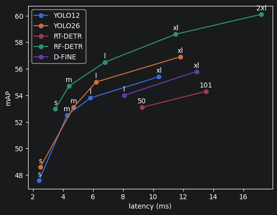
Here is a visualization of the above results alongside additional modern object detection models for a more holistic comparison:
Use-case guidance
Occluded objects: RF-DETR (M/L) is the clear choice. Its DINOv2 backbone models global context across the full image, making it significantly better than CNN-based models at finding partially hidden objects.
Small objects: RF-DETR uses multi-scale feature extraction. YOLO26 also includes STAL (small-target-aware label assignment), making it competitive for small objects on edge hardware.
Edge / mobile / Jetson: YOLO26-N or YOLO12-N. YOLO26 is the Ultralytics recommendation for Jetson Orin/Xavier, Snapdragon AI, and ARM CPUs. It has 43% faster CPU inference than YOLO11n at comparable accuracy.
Custom domain / fine-tuning: RF-DETR by a significant margin. DINOv2 pre-training means it adapts to new domains (medical, aerial, and industrial) faster and with less data than any other model here.
Licensing Summary
| Model | License | Commercial use |
|---|---|---|
| RF-DETR (base) | Apache 2.0 | Free for all uses, including commercial products |
| RF-DETR XL/2XL | PML 1.0 | Contact Roboflow for commercial licensing |
| YOLO12 | AGPL-3.0 | Free for open source / personal use; commercial applications require an Ultralytics Enterprise license |
| YOLO26 | AGPL-3.0 | Free for open source / personal use; commercial applications require an Ultralytics Enterprise license |
Quick-start code
RF-DETR
# Install
pip install rfdetr

# Inference
from rfdetr import RFDETRBase
model = RFDETRBase()
detections = model.predict("image.jpg")

# Fine-tune on your dataset
model.train(dataset_dir="./my_dataset", epochs=50, batch_size=4)
YOLO26 / YOLO12 (via Ultralytics)
# Install
pip install ultralytics

# Inference — YOLO26
from ultralytics import YOLO
model = YOLO("yolo26n.pt")          # or yolo26s/m/l/x
results = model.predict("image.jpg")

# Inference — YOLO12
model = YOLO("yolo12n.pt")
results = model.predict("image.jpg")

# Export for edge (TensorRT / CoreML / ONNX)
model.export(format="engine")       # TensorRT for Jetson
model.export(format="coreml")       # Apple Silicon / iOS
model.export(format="tflite")       # Android / ARM
YOLO12 (use original open-source repo – not the Ultralytics integration)
# Install from the original authors' repo
conda create -n yolov12 python=3.11
conda activate yolov12
git clone https://github.com/sunsmarterjie/yolov12 && cd yolov12
pip install -r requirements.txt
pip install -e .

# Inference
from ultralytics import YOLO
model = YOLO("yolov12n.pt")         # or s/m/l/x
results = model("path/to/image.jpg")
results[0].show()

# Export for edge
model.export(format="engine", half=True)   # TensorRT FP16
model.export(format="onnx")                # ONNX for broad compatibility
Transfer learning and fine-tuning
RF-DETR – recommended for domain shift. Thanks to a DINOv2 backbone that is pre-trained on internet-scale data, fine-tuning requires less labeled data and converges faster. Use the rfdetr package with a COCO pre-trained checkpoint. Roboflow also offers a hosted fine-tuning UI.
YOLO26 / YOLO12 – easiest pipeline. Ultralytics’ training API is the most mature fine-tuning ecosystem. It supports YOLO-format and COCO-format datasets and has good documentation and an active community.
# Fine-tuning YOLO26 on a custom dataset (YOLO format)
from ultralytics import YOLO

model = YOLO("yolo26m.pt")          # start from pretrained weights
model.train(
    data="custom_dataset.yaml",     # path to your dataset config
    epochs=100,
    imgsz=640,
    batch=16,
    device=0,                       # GPU index; "cpu" for CPU
)
metrics = model.val()               # evaluate on validation set
Summary: Choosing the right model for your project
Selecting an object detection model requires matching your specific requirements against each model’s strengths. The decision framework below maps common scenarios to optimal model choices.
| Your goal | Best choice | Runner-up |
|---|---|---|
| Highest accuracy, cloud deployment | RF-DETR M/XL | YOLO26-X |
| Edge / Jetson / mobile | YOLO26-N/S | YOLO12-N |
| Fine-tuning on a custom domain | RF-DETR | YOLO26 |
| Occluded / complex scenes | RF-DETR | YOLO26 |
| Research / benchmarking | YOLO12 | RF-DETR |
| Apache 2.0 + commercial use | RF-DETR (base) | YOLO26 |
| Multi-task (detect + segment + pose) | YOLO26 | RF-DETR (det+seg) |
Get started with PyCharm today
Selecting an object detection architecture in 2026 is a strategic decision dictated by the specific requirements of the application and the available computational budget. Whether prioritizing the record-breaking accuracy of RF-DETR for complex scenes or the unmatched efficiency of the YOLO family for edge deployment, the choice must balance mAP requirements against real-time latency constraints.
The landscape of computer vision is rapidly shifting toward zero-shot detection frameworks that recognize novel objects without task-specific supervision. As foundation models increasingly integrate sophisticated image embedders like CLIP or DINOv2 into detection pipelines, the boundaries of high-precision detection on resource-constrained hardware will continue to expand. While transformer-based architectures are developing quickly, the YOLO family’s established ecosystem ensures it remains a cornerstone for real-time production environments.
To achieve the best results for your specific use case, we encourage you to experiment with the models and code samples provided in this guide. To that end, PyCharm provides the perfect ecosystem for experimentation with various open-source models via Code -> Insert HF Model interface. If you’d like to try this yourself, PyCharm Pro comes with a 30-day trial.
For a hands-on starting point, this tutorial shows how to build a live object detection app using TensorFlow and PyCharm Jupyter notebooks, then deploy it on a robot – covering everything from single-frame inference to a live web dashboard with annotated detections. Moreover, stay tuned for the next tutorial post, where we will discuss all three object detection models in action.