How to Train Your First TensorFlow Model in PyCharm

This is a guest post from Iulia Feroli, founder of the Back To Engineering community on YouTube.
TensorFlow is a powerful open-source framework for building machine learning and deep learning systems. At its core, it works with tensors (a.k.a multi‑dimensional arrays) and provides high‑level libraries (like Keras) that make it easy to transform raw data into models you can train, evaluate, and deploy.
TensorFlow helps you handle the full pipeline: loading and preprocessing data, assembling models from layers and activations, training with optimizers and loss functions, and exporting for serving or even running on edge devices (including lightweight TensorFlow Lite models on Raspberry Pi and other microcontrollers).
If you want to make data-driven applications, prototyping neural networks, or ship models to production or devices, learning TensorFlow gives you a consistent, well-supported toolkit to go from idea to deployment.
If you’re brand new to TensorFlow, start by watching the short overview video where I explain tensors, neural networks, layers, and why TensorFlow is great for taking data → model → deployment, and how all of this can be explained with a LEGO-style pieces sorting example.
In this blog post, I’ll walk you through a first, stripped-down TensorFlow implementation notebook so we can get started with some practical experience. You can also watch the walkthrough video to follow along.
We’ll be exploring a very simple use case today: load the Fashion MNIST dataset, build two very simple Keras models, train and compare them, then dig into visualizations (predictions, confidence bars, confusion matrix). I kept the code minimal and readable so you can focus on the ideas – and you’ll see how PyCharm helps along the way.
Training TensorFlow models step by step
Getting started in PyCharm
We’ll be leveraging PyCharm’s native Notebook integration to build out our project. This way, we can inspect each step of the pipeline and use some supporting visualization along the way. We’ll create a new project and generate a virtual environment to manage our dependencies.
If you’re running the code from the attached repo, you can install directly from the requirements file. If you wish to expand this example with additional visualizations for further models, you can easily add more packages to your requirements as you go by using the PyCharm package manager helpers for installing and upgrading.
Load Fashion MNIST and inspect the data
Fashion MNIST is a great starter because the images are small (28×28 pixels), visually meaningful, and easy to interpret. They represent various garment types as pixelated black-and-white images, and provide the relevant labels for a well-contained classification task. We can first take a look at our data sample by printing some of these images with various matplotlib functions:
```
fig, axes = plt.subplots(2, 5, figsize=(10, 4))
for i, ax in enumerate(axes.flat):
    ax.imshow(x_train[i], cmap='gray')
    ax.set_title(class_names[y_train[i]])
    ax.axis('off')
plt.show()
```
# Two simple models (a quick experiment)
```
model1 = models.Sequential([
    layers.Flatten(input_shape=(28, 28)),
    layers.Dense(128, activation='relu'),
    layers.Dense(10, activation='softmax')
])
model2 = models.Sequential([
    layers.Flatten(input_shape=(28, 28)),
    layers.Dense(128, activation='relu'),
    layers.Dense(128, activation='relu'),
    layers.Dense(10, activation='softmax')
])
```
Compile and train your first model
From here, we can compile and train our first TensorFlow model(s). With PyCharm’s code completion features and documentation access, you can get instant suggestions for building out these simple code blocks.
For a first try at TensorFlow, this allows us to spin up a working model with just a few presses of Tab in our IDE. We’re using the recommended standard optimizer and loss function, and we’re tracking for accuracy. We can choose to build multiple models by playing around with the number or type of layers, along with the other parameters.
```
model1.compile(
    optimizer='adam',
    loss='sparse_categorical_crossentropy',
    metrics=['accuracy']
)
model1.fit(x_train, y_train, epochs=10)
model2.compile(
    optimizer='adam',
    loss='sparse_categorical_crossentropy',
    metrics=['accuracy']
)
model2.fit(x_train, y_train, epochs=15)
```
Evaluate and compare your TensorFlow model performance
```
loss1, accuracy1 = model1.evaluate(x_test, y_test)
print(f'Accuracy of model1: {accuracy1:.2f}')
loss2, accuracy2 = model2.evaluate(x_test, y_test)
print(f'Accuracy of model2: {accuracy2:.2f}')
```
Once the models are trained (and you can see the epochs progressing visually as each cell is run), we can immediately evaluate the performance of the models.
In my experiment, model1 sits around ~0.88 accuracy, and while model2 is a little higher than that, it took 50% longer to train. That’s the kind of trade‑off you should be thinking about: Is a tiny accuracy gain worth the additional compute and complexity?
We can dive further into the results of the model run by generating a DataFrame instance of our new prediction dataset. Here we can also leverage built-in functions like `describe` to quickly get some initial statistical impressions:
```
predictions = model1.predict(x_test)
import pandas as pd
df_pred = pd.DataFrame(predictions, columns=class_names)
df_pred.describe()
```
However, the most useful statistics will compare our model’s prediction with the ground truth “real” labels of our dataset. We can also break this down by item category:
```
y_pred = model1.predict(x_test).argmax(axis=1)
cm = confusion_matrix(y_test, y_pred)
plt.figure(figsize=(8,6))
sns.heatmap(cm, annot=True, fmt='d', cmap='Blues', xticklabels=class_names, yticklabels=class_names)
plt.xlabel('Predicted')
plt.ylabel('True')
plt.title('Confusion Matrix')
plt.show()
print('Classification report:')
print(classification_report(y_test, y_pred, target_names=class_names))
```
From here, we can notice that the accuracy differs quite a bit by type of garment. A possible interpretation of this is that trousers are quite a distinct type of clothing from, say, t-shirts and shirts, which can be more commonly confused.
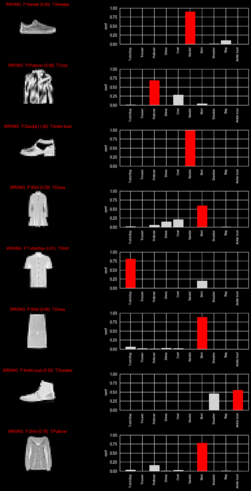
This is, of course, the type of nuance that, as humans, we can pick up by looking at the images, but the model only has access to a matrix of pixel values. The data does seem, however, to confirm our intuition. We can further build a more comprehensive visualization to test this hypothesis.
```
import numpy as np
import matplotlib.pyplot as plt
# pick 8 wrong examples
y_pred = predictions.argmax(axis=1)
wrong_idx = np.where(y_pred != y_test)[0][:8]  # first 8 mistakes
n = len(wrong_idx)
fig, axes = plt.subplots(n, 2, figsize=(10, 2.2 * n), constrained_layout=True)
for row, idx in enumerate(wrong_idx):
    p = predictions[idx]
    pred = int(np.argmax(p))
    true = int(y_test[idx])
    axes[row, 0].imshow(x_test[idx], cmap="gray")
    axes[row, 0].axis("off")
    axes[row, 0].set_title(
        f"WRONG  P:{class_names[pred]} ({p[pred]:.2f})  T:{class_names[true]}",
        color="red",
        fontsize=10
    )
    bars = axes[row, 1].bar(range(len(class_names)), p, color="lightgray")
    bars[pred].set_color("red")
    axes[row, 1].set_ylim(0, 1)
    axes[row, 1].set_xticks(range(len(class_names)))
    axes[row, 1].set_xticklabels(class_names, rotation=90, fontsize=8)
    axes[row, 1].set_ylabel("conf", fontsize=9)
plt.show()
```
This table generates a view where we can explore the confidence our model had in a prediction: By exploring which weight each class was given, we can see where there was doubt (i.e. multiple classes with a higher weight) versus when the model was certain (only one guess). These examples further confirm our intuition: top-types appear to be more commonly confused by the model.
Conclusion
And there we have it! We were able to set up and train our first model and already drive some data science insights from our data and model results. Using some of the PyCharm functionalities at this point can speed up the experimentation process by providing access to our documentation and applying code completion directly in the cells. We can even use AI Assistant to help generate some of the graphs we’ll need to further evaluate the TensorFlow model performance and investigate our results.
You can try out this notebook yourself, or better yet, try to generate it with these same tools for a more hands-on learning experience.
Where to go next
This notebook is a minimal, teachable starting point. Here are some practical next steps to try afterwards:
- Replace the dense baseline with a small CNN (Conv2D → MaxPooling → Dense).
- Add dropout or batch normalization to reduce overfitting.
- Apply data augmentation (random shifts/rotations) to improve generalization.
- Use callbacks like
EarlyStoppingandModelCheckpointso training is efficient, and you keep the best weights. - Export a
SavedModelfor server use or convert to TensorFlow Lite for edge devices (Raspberry Pi, microcontrollers).
Frequently asked questions
When should I use TensorFlow?
TensorFlow is best used when building machine learning or deep learning models that need to scale, go into production, or run across different environments (cloud, mobile, edge devices).
TensorFlow is particularly well-suited for large-scale models and neural networks, including scenarios where you need strong deployment support (TensorFlow Serving, TensorFlow Lite). For research prototypes, TensorFlow is viable, but it’s more commonplace to use lightweight frameworks for easier experimentation.
Can TensorFlow run on a GPU?
Yes, TensorFlow can run GPUs and TPUs. Additionally, using a GPU can significantly speed up training, especially for deep learning models with large datasets. The best part is, TensorFlow will automatically use an available GPU if it’s properly configured.
What is loss in TensorFlow?
Loss (otherwise known as loss function) measures how far a model’s predictions are from the actual target values. Loss in TensorFlow is a numerical value representing the distance between predictions and actual target values. A few examples include:
- MSE (mean squared error), used in regression tasks.
- Cross-entropy loss, often used in classification tasks.
How many epochs should I use?
There’s no set number of epochs to use, as it depends on your dataset and model. Typical approaches cover:
- Starting with a conservative number (10–50 epochs).
- Monitoring validation loss/accuracy and adjusting based on the results you see.
- Using early stopping to halt training when improvements decrease.
An epoch is one full pass through your training data. Not enough passes through leads to underfitting, and too many can cause overfitting. The sweet spot is where your model generalizes best to unseen data.
About the author