Euro 2024: Scoring Goals With Python

Regina Muradova

Now that the 2024 UEFA European Football Championship is over, and we’ve all experienced the thrilling moments of cheering for our favorite teams, let’s have some fun with Python and dive into the tournament’s data. Why not combine our love for football with some cool data analysis?

In this blog post, we’ll demonstrate how Python works by exploring data from Euro 2024. Not only will we gain new insights about Europe’s premier sporting event, but we’ll also show you how to use Python for basic data analysis in real-world scenarios. And you may just find that data analysis can be as fun as the game itself.

Preparing the data

First, we need to set up our environment and load the data. The data for this analysis is sourced from the Euro 2024 dataset available from Kaggle. We took the 2024.csv file from the matches | euro tab.

For this analysis, we’ll be using PyCharm. Either PyСharm Community Edition (completely free) or PyСharm Professional (available with a 30-day free trial) will be fine. Once you’ve downloaded the IDE, open it up, start a new project, and put the CSV file into the project folder. Make sure the matplotlib and numpy libraries are installed in your IDE.

We’ll run the code in Jupyter Notebook (available only in PyCharm Professional), but you can also run the code directly in PyCharm without the notebook—it’s entirely up to you.

import csv
import matplotlib.pyplot as plt
import numpy as np
import matplotlib
matplotlib.use('TkAgg')

CSV_PATH = '2024.csv'

def load_csv(csv_path):
   """Load a CSV file and return two lists: events and players"""
   events = []
   players = []

   with open(csv_path, encoding='latin-1') as csv_f:
       fixed_data = csv_f.read().replace(' nan', ' None')  # Preprocess data from csv-file
       reader = csv.reader(fixed_data.splitlines())

       headers = next(reader)  # Skip the header
       for row in reader:
           events += eval(row[-1])
           players += eval(row[-4])  # Add teams from "home" games
           players += eval(row[-5])  # Add teams from "away" games

   # So far, the "players" list contains multiple copies of the same players from different games;
   # Fix it by putting the players into a dictionary by ID, thus overwriting duplicates
   players_dict = {i['id_player']: i for i in players}
   players = players_dict.values()

   # We're only interested in events related to a person (e.g. "goal", "card"). Remove the rest
   events = [i for i in events if i['primary_id_person'] is not None]

   return events, players


def find_player_by_id(players, player_id):
   """Return the player corresponding to the specified player ID"""
   return [i for i in players if i['id_player'] == player_id][0]


def filter_events_by_type(all_events, event_type):
   """Return a list of events with only a given type (e.g. 'GOAL')"""
   return [i for i in all_events if i['type'] == event_type]

Now let’s run the function def load_csv(csv_path) to load data from the file:

events, players = load_csv(CSV_PATH)

We have loaded the data about events and players, and it’s now ready for analysis.

Most valuable body part

Ever wondered whether players score more with their head, right foot, or left foot? To kick off our analysis, we broke down goals by body parts. We collected the data and visualized it in a pie chart to see which body parts are the true game-changers on the field.

Counting goals by body part

def count_goals_by_body_part(goal_events):
    """Take goal events and count the number of goals per body part; return as a dict"""
    result = {}
    for event in goal_events:
        body_part = event.get('body_part')
        if body_part:
            result[body_part] = result.get(body_part, 0) + 1
    return result

Displaying the pie chart

def show_body_part_pie_chart(body_parts_count):
    """Plot and show a pie chart of goals by body part"""
    colors = ['#AE1DF4', '#01E08F', '#7463FF', '#111111']
    
    plt.figure(figsize=(6, 6), dpi=130)
    plt.pie(
        body_parts_count.values(),
        labels=body_parts_count.keys(),
        autopct='%1.1f%%',
        textprops={'color': '#333333'},
        colors=colors[:len(body_parts_count)]  # Adjust colors list length
    )
    plt.title('Goals per body part')
    plt.show()

Running the functions

goal_events = filter_events_by_type(events, 'GOAL')
body_parts_count = count_goals_by_body_part(goal_events)
show_body_part_pie_chart(body_parts_count)

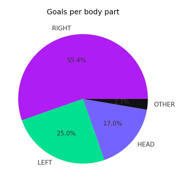
Our analysis showed some expected results, with right-footed goals being the most common. However, it also revealed that left-footed goals were more frequent than headers, showing that in football, each of these body parts can make a difference when it comes to scoring goals.

Watch the demo to see how this code runs in the IDE. 👇🏻

Goals and yellow cards by jersey numbers

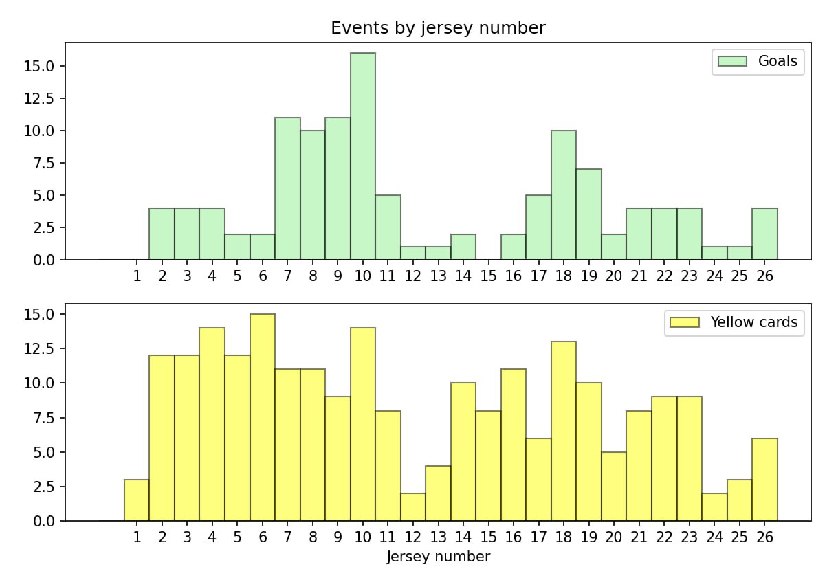
Next, we looked at goals scored by players based on their jersey numbers. Do players with certain numbers tend to score more goals? Let’s find out.

Preparing the functions

def get_jerseys_numbers_by_event(events, players, event_type):
    """Return a simple list of jersey numbers corresponding to events of specified event_type"""
 
    selected_events = filter_events_by_type(events, event_type)
 
    # Helper function to find a player by ID and return his number
    def jersey_num_by_id(player_id):
        return find_player_by_id(players, player_id)['jersey_namber']
 
    return [jersey_num_by_id(i['primary_id_person']) for i in selected_events]
 
 
def plot_jerseys_numbers_histogram(jerseys_list, data_label, data_color):
    '''Plot the jersey histogram based on "jerseys_list" data'''
    MAX_JERSEY_NUM = 26
    _, bins, _ = plt.hist(
        jerseys_list,
        bins=np.arange(MAX_JERSEY_NUM + 2) - 0.5,
        label=data_label,
        edgecolor='black',
        color=data_color,
        alpha=0.5
    )
    plt.xticks(0.5 * (bins[1:-1] + bins[2:]))  # Make sure all numbers are labeld on x-axis
    plt.legend()

Running the functions and displaying the histograms

goals_jerseys = get_jerseys_numbers_by_event(events, players, 'GOAL')
cards_jerseys = get_jerseys_numbers_by_event(events, players, 'YELLOW_CARD')
 
plt.subplot(2, 1, 1)  # Top plot
plt.title('Events by jersey number')
plot_jerseys_numbers_histogram(goals_jerseys, 'Goals', 'lightgreen')
 
plt.subplot(2, 1, 2)  # Bottom plot
plt.xlabel('Jersey number')
plot_jerseys_numbers_histogram(cards_jerseys, 'Yellow cards', 'yellow')
 
plt.show()

Watch the demo to see how this code runs in the IDE. 👇🏻

Our analysis revealed that players wearing the number 10 jersey scored the most goals. Legends like Pelé, Maradona, and Messi all wore this iconic number, demonstrating that the greatest forwards truly prefer number 10.

We also looked at which jersey numbers get the most yellow cards. Defenders wearing numbers like 4 and 6 rack them up the most. Are defensive responsibilities more likely to land you on the wrong side of the ref’s whistle? Or do players with a penchant for flouting the rules simply gravitate toward defense? It’s hard to say from these numbers alone.

Numbers like 1, 12, and 24 show up less frequently for both goals and yellow cards. This could be due to these numbers often being worn by goalkeepers.

Using Python, we visualized these trends with histograms. Some numbers, like 10, stand out with scoring goals, while others, like 4 and 6, handle the tougher tasks on the field.

Goals by zodiac signs

And finally, we thought it would be fun to see if Python could tell us anything about football players based on their zodiac signs. Could the stars really predict on-field actions? In this playful experiment, we mixed astrology with football to find out.

We started by calculating the zodiac sign for each player using their birth date. Then, we looked at how often players with different signs scored goals or received yellow cards. After adjusting for the overall distribution of zodiac signs among players in each game, we visualized the data with some cool histograms. We won’t dive into the code details here—instead, we invite you to simply enjoy the chart.

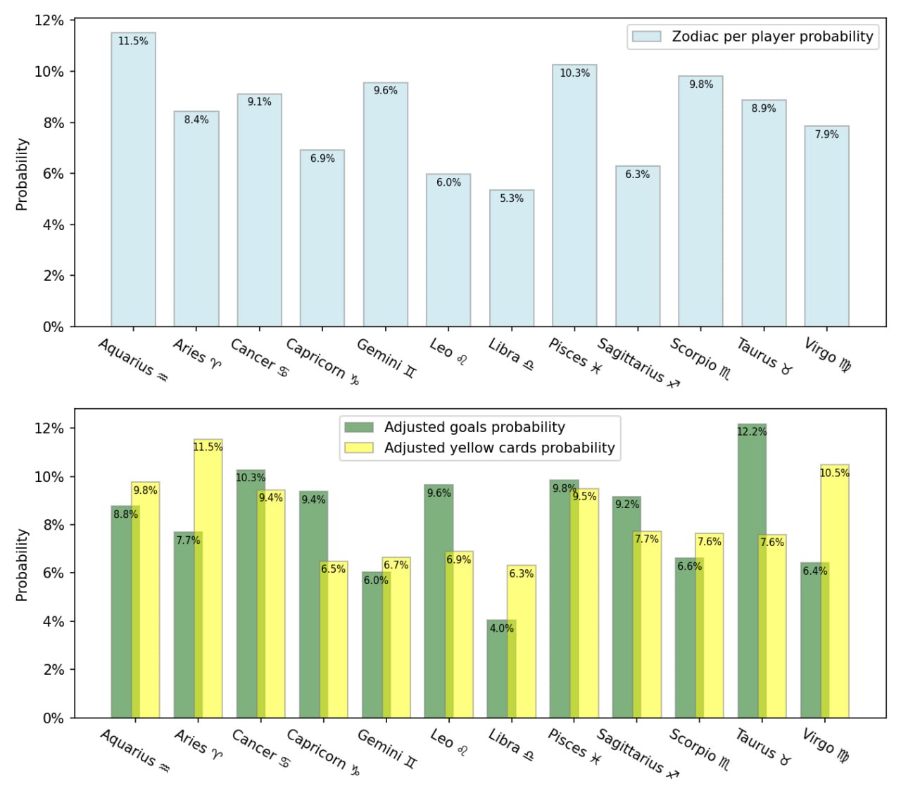
Take a look at your sign on the chart – do the stats align with its profile? Taurus players, who are known for being determined and steady, seem to score the most goals. On the other hand, Aries, with their fiery and bold nature, are leading in yellow cards.

As you can see, there’s no limit to the types of interesting insights you can uncover with Python and data science. If football isn’t your thing, what other data would you like to analyze with Python? 

If you also want to try Python, you can dive into our new Football Analysis project, where you’ll get hands-on experience analyzing football data. Or if you are eager to learn data analysis and kickstart your career in this field, explore our Data Analyst course on Hyperskill. You’ll learn how to handle, visualize, and interpret data effectively. For a deeper understanding of data analysis, consider adding Introduction to Data Science to your portfolio.

Happy learning!

Your JetBrains Academy team

Note: The data used in this analysis is for educational purposes only and is not intended to bring JetBrains commercial advantage or monetary compensation. For further use of any data mentioned in this post, please always ensure you comply with the relevant license terms.

Subscribe to JetBrains Academy updates

Subscribe form

By submitting this form, I agree to the JetBrains Privacy Policy Notification icon

By submitting this form, I agree that JetBrains s.r.o. ("JetBrains") may use my name, email address, and location data to send me newsletters, including commercial communications, and to process my personal data for this purpose. I agree that JetBrains may process said data using third-party services for this purpose in accordance with the JetBrains Privacy Policy. I understand that I can revoke this consent at any time in my profile. In addition, an unsubscribe link is included in each email.

Submit

Thanks, we've got you!