How to Do Sentiment Analysis With Large Language Models

Sentiment analysis is a powerful tool for understanding emotions in text. While there are many ways to approach sentiment analysis, including more traditional lexicon-based and machine learning approaches, today we’ll be focusing on one of the most cutting-edge ways of working with text – large language models (LLMs). We’ll explain how you can use these powerful models to predict the sentiment expressed in a text.
As a practical tutorial, this post will introduce you to the types of LLMs most suited for sentiment analysis tasks and then show you how to choose the right model for your specific task.
We’ll cover using models that other people have fine-tuned for sentiment analysis and how to fine-tune one yourself. We’ll also look at some of the powerful tools and resources available that can help you work with these models easily, while demystifying what can feel like an overly complex and overwhelming topic.
To get the most out of this blog post, we’d recommend you have some experience training machine learning or deep learning models and be confident using Python. Our introductory blog post on sentiment analysis with Python is a great place to begin. That said, you don’t necessarily need to have a background in large language models to enjoy it.
Let’s get started!
What are large language models?
Large language models are some of the latest and most powerful tools for solving natural language problems. In brief, they are generalist language models that can complete a range of natural language tasks, from named entity recognition to question answering. LLMs are based on the transformer architecture, a type of neural network that uses a mechanism called attention to represent complex and nuanced relationships between words in a piece of text. This design allows LLMs to accurately represent the information being conveyed in a piece of text.
The full transformer model architecture consists of two blocks. Encoder blocks are designed to receive text inputs and build a representation of them, creating a feature set based on the text corpus over which the model is trained. Decoder blocks take the features generated by the encoder and other inputs and attempt to generate a sequence based on these.
Transformer models can be divided up based on whether they contain encoder blocks, decoder blocks, or both.
- Encoder-only models tend to be good at tasks requiring a detailed understanding of the input to do downstream tasks, like text classification and named entity recognition.
- Decoder-only models are best for tasks such as text generation.
- Encoder-decoder, or sequence-to-sequence models are mainly used for tasks that require the model to evaluate an input and generate a different output, such as translation. In fact, translation was the original task that transformer models were designed for!
This Hugging Face table (also featured below), which I took from their course on natural language processing, gives an overview of what each model tends to be strongest at.
After finishing this blog post and discovering what other natural language tasks you can perform with the Transformers library, I recommend the course if you’d like to learn more about LLMs. It strikes an excellent balance between accessibility and technical depth.
| Model type | Examples | Tasks |
| Encoder-only | ALBERT, BERT, DistilBERT, ELECTRA, RoBERTa | Sentence classification, named entity recognition, extractive question answering |
| Decoder-only | CTRL, GPT, GPT-2, Transformer XL | Text generation |
| Encoder-decoder | BART, T5, Marian, mBART | Summarization, translation, generative question answering |
Sentiment analysis is usually treated as a text or sentence classification problem with LLMs, meaning that encoder-only models such as RoBERTa, BERT, and ELECTRA are most often used for this task. However, there are some exceptions. For example, the top scoring model for aspect-based sentiment analysis, InstructABSA, is based on a fine-tuned version of T5, an encoder-decoder model.
Using large language models for sentiment analysis
With all of the background out of the way, we can now get started with using LLMs to do sentiment analysis.
Install PyCharm to get started with sentiment analysis
We’ll use PyCharm Professional for this demo, but you can follow along with any other IDE that supports Python development.
PyCharm Professional is a powerful Python IDE for data science. It supports advanced Python code completion, inspections and debugging, rich databases, Jupyter, Git, Conda, and more right out of the box. You can try out great features such as our DataFrame Column Statistics and Chart View, as well as Hugging Face integrations, which make working with LLMs much simpler and faster.
If you’d like to follow along with this tutorial, you can activate your free three-month subscription to PyCharm using this special promo code: PCSA24. Click on the link below, and enter the code. You’ll then receive an activation code through your email.
Import the required libraries
There are two parts to this tutorial: using an LLM that someone else has fine-tuned for sentiment analysis, and fine-tuning a model ourselves.
In order to run both parts of this tutorial, we need to import the following packages:
- Transformers: As described, this will allow us to use fine-tuned LLMs for sentiment analysis and fine-tune our own models.
- PyTorch, Tensorflow, or Flax: Transformers acts as a high-level interface for deep learning frameworks, reusing their functionality for building, training, and running neural networks. In order to actually work with LLMs using the Transformers package, you will need to install your choice of PyTorch, Tensorflow, or Flax. PyTorch supports the largest number of models of the three frameworks, so that’s the one we’ll use in this tutorial.
- Datasets: This is another package from Hugging Face that allows you to easily work with the datasets hosted on Hugging Face Hub. We’ll need this package to get a dataset to fine-tune an LLM for sentiment analysis.
In order to fine-tune our own model, we also need to import these additional packages:
- NumPy: NumPy allows us to work with arrays. We’ll need this to do some post-processing on the predictions generated by our LLM.
- scikit-learn: This package contains a huge range of functionality for machine learning. We’ll use it to evaluate the performance of our model.
- Evaluate: This is another package from Hugging Face. Evaluate adds a convenient interface for measuring the performance of models. It will give us an alternative way of measuring our model’s performance.
- Accelerate: This final package from Hugging Face, Accelerate, takes care of distributed model training.
We can easily find and install these in PyCharm. Make sure you’re using a Python 3.7 or higher interpreter. For this demo, we’ll be using Python 3.11.7.

Pick the right model
The next step is picking the right model. Before we get into that, we need to cover some terminology.
LLMs are made up of two components: an architecture and a checkpoint. The architecture is like the blueprint of the model, and describes what will be contained in each layer and each operation that takes place within the model.
The checkpoint refers to the weights that will be used within each layer. Each of the pretrained models will use an architecture like T5 or GPT, and obtain the specific weights (the model checkpoint) by training the model over a huge corpus of text data.
Fine-tuning will adjust the weights in the checkpoint by retraining the last layer(s) on a dataset specialized in a certain task or domain. To make predictions (called inference), an architecture will load in the checkpoint and use this to process text inputs, and together this is called a model.
If you’ve ever looked at the models available on Hugging Face, you might have been overwhelmed by the sheer number of them (even when we narrow them down to encoder-only models).
So, how do you know which one to use for sentiment analysis?
One useful place to start is the sentiment analysis page on Papers With Code. This page includes a very helpful overview of this task and a Benchmarks table that includes the top-performing models for each sentiment analysis benchmarking dataset. From this page, we can see that some of the commonly appearing models are those based on BERT and RoBERTa architectures.
While we may not be able to access these exact model checkpoints on Hugging Face (as not all of them will be uploaded there), it can give us a guide for what sorts of models might perform well at this task. Papers With Code also has similar pages for a range of other natural language tasks: If you search for the task in the upper left-hand corner of the site, you can navigate to these.
Now that we know what kinds of architectures are likely to do well for this problem, we can start searching for a specific model.
PyCharm has an built-in integration with Hugging Face that allows us to search for models directly. Simply right-click anywhere in your Jupyter notebook or Python script, and select Insert HF model. You’ll be presented with the following window:
You can see that we can find Hugging Face models either by the task type (which we can select from the menu on the left-hand side), by keyword search in the search box at the top of the window, or by a combination of both. Models are ranked by the number of likes by default, but we can also select models based on downloads or when the model was created or last modified.
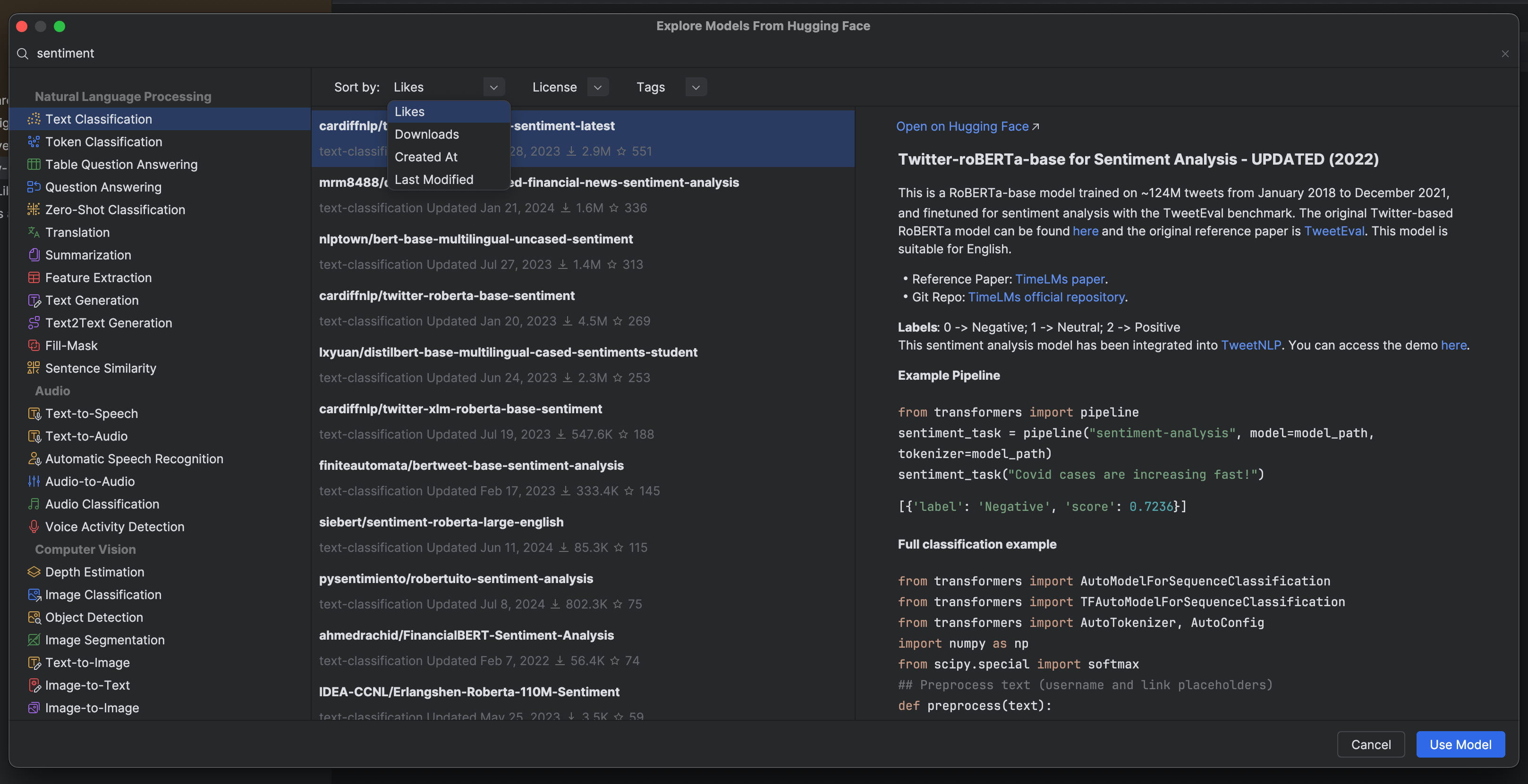
When you use a model for a task, the checkpoint is downloaded and cached, making it faster the next time you need to use that model. You can see all of the models you’ve downloaded in the Hugging Face tool window.
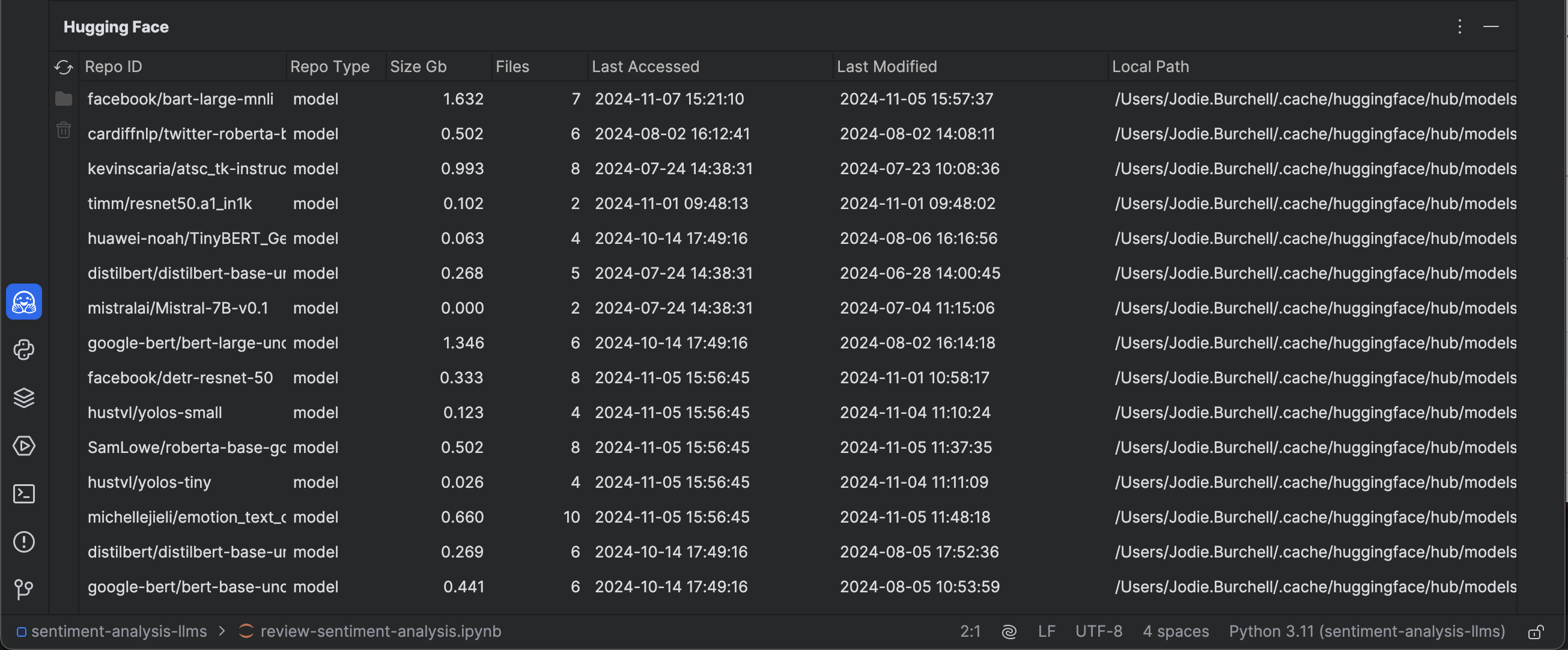
Once we’ve downloaded the model, we can also look at its model card again by hovering over the model name in our Jupyter notebook or Python script. We can do the same thing with dataset cards.
Use a fine-tuned LLM for sentiment analysis
Let’s move on to how we can use a model that someone else has already fine-tuned for sentiment analysis.
As mentioned, sentiment analysis is usually treated as a text classification problem for LLMs. This means that in our Hugging Face model selection window, we’ll select Text Classification, which can be found under Natural Language Processing on the left-hand side. To narrow the results down to sentiment analysis models, we’ll type “sentiment” in the search box in the upper left-hand corner.
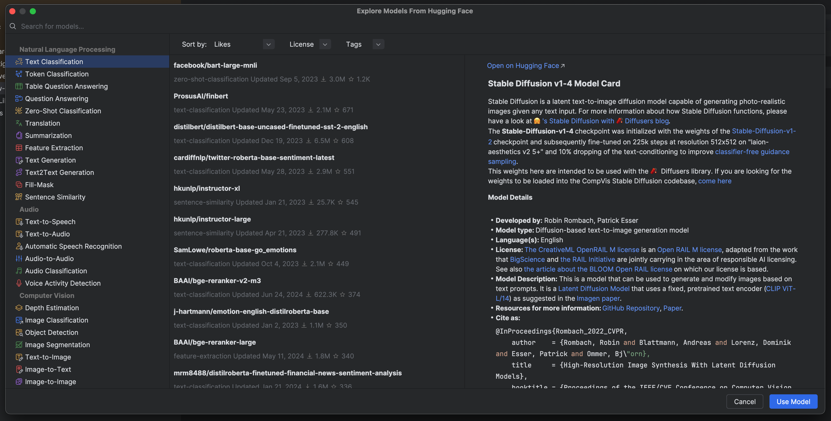
We can see various fine-tuned models, and as expected from what we saw on the Papers With Code Benchmarks table, most of them use RoBERTa or BERT architectures. Let’s try out the top ranked model, Twitter-roBERTa-base for Sentiment Analysis.
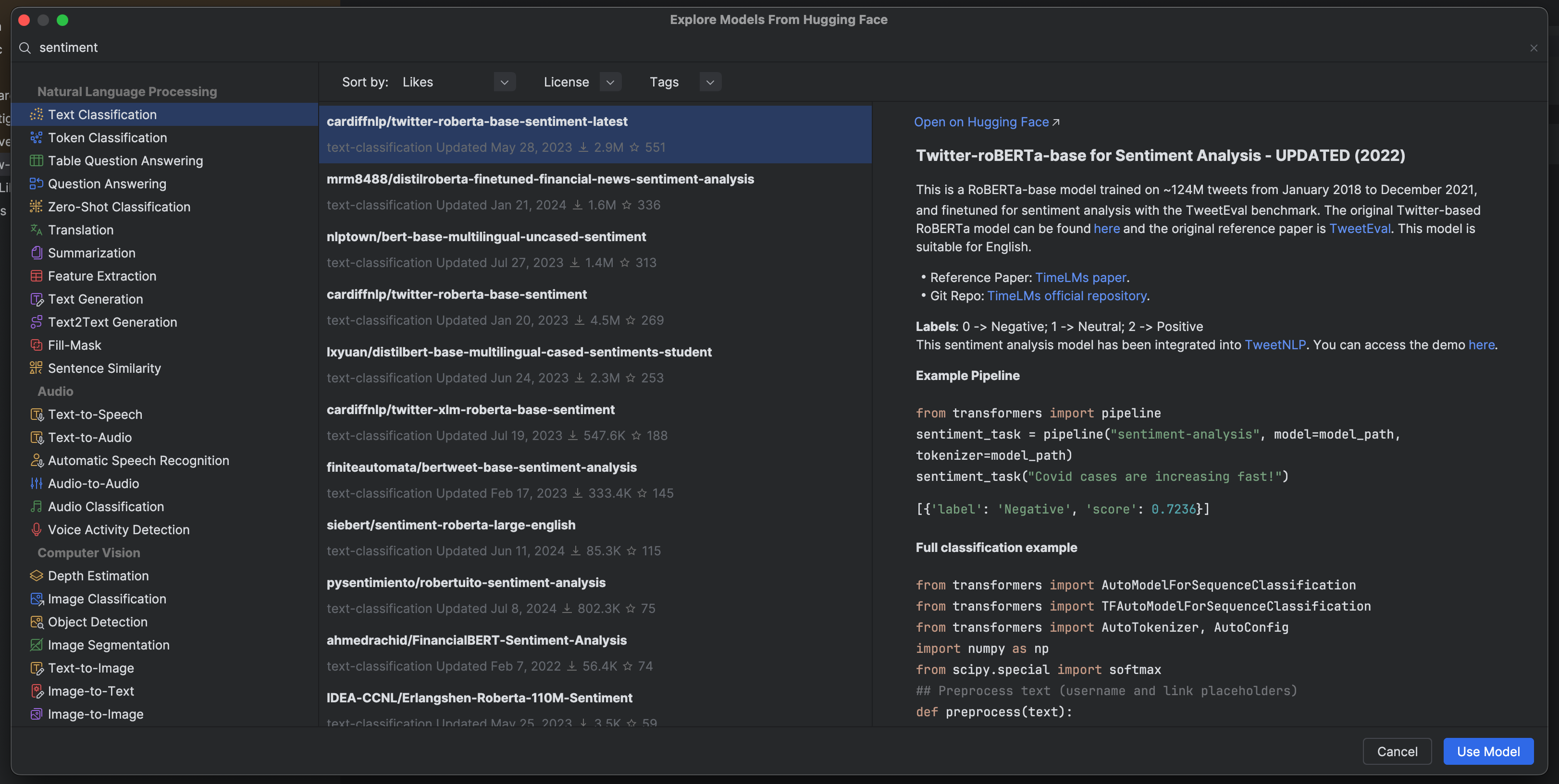
You can see that after we select Use Model in the Hugging Face model selection window, code is automatically generated at the caret in our Jupyter notebook or Python script to allow us to start working with this model.
from transformers import pipeline
pipe = pipeline("text-classification",
 model="cardiffnlp/twitter-roberta-base-sentiment-latest")
Before we can do inference with this model, we’ll need to modify this code.
The first thing we can check is whether we have a GPU available, which will make the model run faster. We’ll check for two types: NVIDIA GPUs, which support CUDA, and Apple GPUs, which support MPS.
import torch
print(f"CUDA available: {torch.cuda.is_available()}")
print(f"MPS available: {torch.backends.mps.is_available()}")
My computer supports MPS, so we can add a device argument to the pipeline and add "mps". If your computer supports CUDA, you can instead add the argument device=0.
from transformers import pipeline

pipe = pipeline("text-classification", model="cardiffnlp/twitter-roberta-base-sentiment-latest",
                device="mps")
Finally, we can get the fine-tuned LLM to run inference over our example text.
result = pipe("I love PyCharm! It's my favorite Python IDE.")
result
[{'label': 'positive', 'score': 0.9914802312850952}]
You can see that this model predicts that the text will be positive, with 99% probability.
Fine-tune your own LLM for sentiment analysis
The other way we can use LLMs for sentiment analysis is to fine-tune our own model.
You might wonder why you’d bother doing this, given the huge number of fine-tuned models that already exist on Hugging Face Hub. The main reason you might want to fine-tune a model is so that you can tailor it to your specific use case.
Most models are fine-tuned on public datasets, especially social media posts and movie reviews, and you might need your model to be more sensitive to your specific domain or use case.
Model fine-tuning can be quite a complex topic, so in this demonstration, I’ll explain how to do it at a more general level. However, if you want to understand this in more detail, you can read more about it in Hugging Face’s excellent NLP course, which I recommended earlier. In their tutorial, they explain in detail how to process data for fine-tuning models and two different approaches to fine-tuning: with the trainer API and without it.
To demonstrate how to fine-tune a model, we’ll use the SST-2 dataset, which is composed of single lines pulled from movie reviews that have been annotated as either negative or positive.
As mentioned earlier, BERT models consistently show up as top performers on the Papers With Code benchmarks, so we’ll fine-tune a BERT checkpoint.
We can again search for these models in PyCharm’s Hugging Face model selection window.
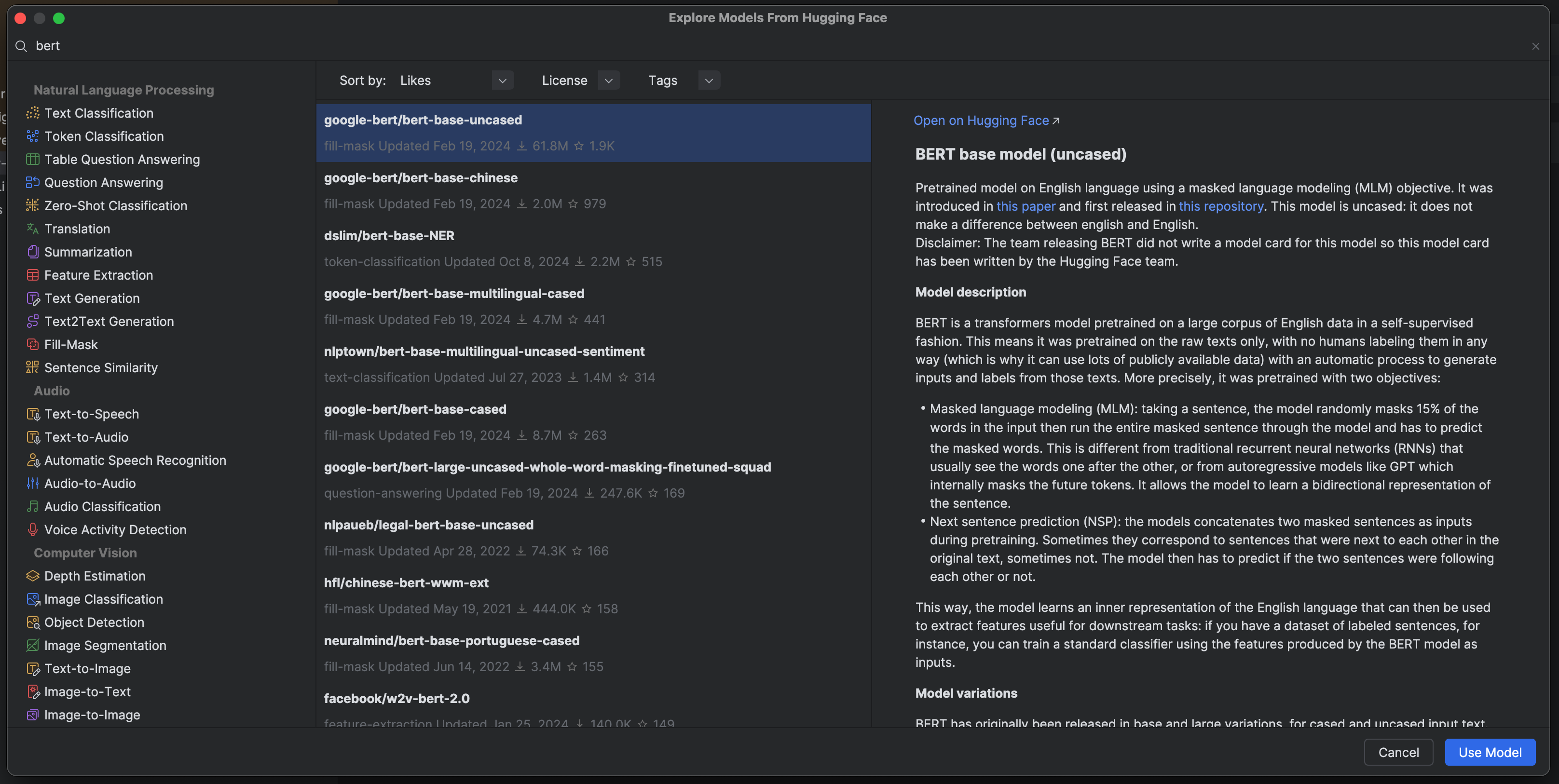
We can see that the most popular BERT model is bert-base-uncased. This is perfect for our use case, as this was also trained on lowercase text, so it will match the casing of our dataset.
We could have used the popular bert-large-uncased, but the base model has only 110 million parameters compared to BERT large, which has 340 million, so the base model is a bit friendlier for fine-tuning on a local machine.
If you still want to use a smaller model, you could also try this with a DistilBERT model, which has far fewer parameters but still preserves most of the performance of the original BERT models.
Let’s start by reading in our dataset. We can do so using the load_dataset() function from the Datasets package. SST-2 is part of the GLUE dataset, which is designed to see how well a model can complete a range of natural language tasks.
from datasets import load_dataset

sst_2_raw = load_dataset("glue", "sst2")
sst_2_raw
DatasetDict({
    train: Dataset({
        features: ['sentence', 'label', 'idx'],
        num_rows: 67349
    })
    validation: Dataset({
        features: ['sentence', 'label', 'idx'],
        num_rows: 872
    })
    test: Dataset({
        features: ['sentence', 'label', 'idx'],
        num_rows: 1821
    })
})
This dataset has already been split into the train, validation, and test sets. We have around 67,349 training examples – quite a modest number for fine-tuning such a large model.
Here’s an example from this dataset.
sst_2_raw["train"][1]
{'sentence': 'contains no wit , only labored gags ', 'label': 0, 'idx': 1}
We can see what the labels mean by calling the features attribute on the training set.
sst_2_raw["train"].features
{'sentence': Value(dtype='string', id=None),
 'label': ClassLabel(names=['negative', 'positive'], id=None),
 'idx': Value(dtype='int32', id=None)}
0 indicates a negative sentiment, and 1 indicates a positive one.
Let’s look at the number in each class:
print(f'Number of negative examples: {sst_2_raw["train"]["label"].count(0)}')
print(f'Number of positive examples: {sst_2_raw["train"]["label"].count(1)}')
Number of negative examples: 29780
Number of positive examples: 37569
The classes in our training data are a tad unbalanced, but they aren’t excessively skewed.
We now need to tokenize our data, transforming the raw text into a form that our model can use. To do this, we need to use the same tokenizer that was used to train the bert-large-uncased model in the first place. The AutoTokenizer class will take care of all of the under-the-hood details for us.
from transformers import AutoTokenizer

checkpoint = "google-bert/bert-base-uncased"
tokenizer = AutoTokenizer.from_pretrained(checkpoint)
Once we’ve loaded in the correct tokenizer, we can apply this to the training data.
tokenised_sentences = tokenizer(sst_2_raw["train"]["sentence"])
Finally, we need to add a function to pad our tokenized sentences. This will make sure all of the inputs in a training batch are the same length – text inputs are rarely the same length and models require a consistent number of features for each input.
from transformers import DataCollatorWithPadding

def tokenize_function(example):
    return tokenizer(example["sentence"])

tokenized_datasets = sst_2_raw.map(tokenize_function, batched=True)
data_collator = DataCollatorWithPadding(tokenizer=tokenizer)
Now that we’ve prepared our dataset, we need to determine how well the model is fitting to the data as it trains. To do this, we need to decide which metrics to use to evaluate the model’s prediction performance.
As we’re dealing with a binary classification problem, we have a few choices of metrics, the most popular of which are accuracy, precision, recall, and the F1 score. In the “Evaluate the model” section, we’ll discuss the pros and cons of using each of these measures.
We have two ways of creating an evaluation function for our model. The first is using the Evaluate package. This package allows us to use the specific evaluator for the SST-2 dataset, meaning we’ll evaluate the model fine-tuning using the specific metrics for this task. In the case of SST-2, the metric used is accuracy.
import evaluate
import numpy as np

def compute_metrics(eval_preds):
    metric = evaluate.load("glue", "sst2")
    logits, labels = eval_preds
    predictions = np.argmax(logits, axis=-1)
    return metric.compute(predictions=predictions, references=labels)
However, if we want to customize the metrics used, we can also create our own evaluation function.
In this case, I’ve imported the accuracy, precision, recall, and F1 score metrics from scikit-learn. I’ve then created a function which takes in the predicted labels versus actual labels for each sentence and calculates the four required metrics. We’ll use this function, as it gives us a wider variety of metrics we can check our model performance against.
from sklearn.metrics import accuracy_score, f1_score, precision_score, recall_score
import numpy as np

def compute_metrics(eval_preds):
    logits, labels = eval_preds
    predictions = np.argmax(logits, axis=-1)
    return {
        'accuracy': accuracy_score(labels, predictions),
        'f1': f1_score(labels, predictions, average='macro'),
        'precision': precision_score(labels, predictions, average='macro'),
        'recall': recall_score(labels, predictions, average='macro')
    }
Now that we’ve done all of the setup, we’re ready to train the model. The first thing we need to do is define some parameters that will control the training process using the TrainingArguments class. We’ve only specified a few parameters here, but this class has an enormous number of possible arguments allowing you to calibrate your model training to a high degree of specificity.
from transformers import TrainingArguments

training_args = TrainingArguments(output_dir="sst2-bert-fine-tuning",
                                  eval_strategy="epoch",
                                  num_train_epochs=3)
In our case, we’ve used the following arguments:
output_dir: The output directory where we want our model predictions and checkpoints saved.eval_strategy="epoch": This ensures that the evaluation is performed at the end of each training epoch. Other possible values are “steps” (meaning that evaluation is done at regular step intervals) and “no” (meaning that evaluation is not done during training).num_train_epochs=3: This sets the number of training epochs (or the number of times the training loop will repeat over all of the data). In this case, it’s set to train on the data three times.
The next step is to load in our pre-trained BERT model.
from transformers import AutoModelForSequenceClassification

model = AutoModelForSequenceClassification.from_pretrained(checkpoint, num_labels=2)
Some weights of BertForSequenceClassification were not initialized from the model checkpoint at google-bert/bert-base-uncased and are newly initialized: ['classifier.bias', 'classifier.weight']
You should probably TRAIN this model on a down-stream task to be able to use it for predictions and inference.
Let’s break this down step-by-step:
- The
AutoModelForSequenceClassificationclass does two things. First, it automatically identifies the appropriate model architecture from the Hugging Face model hub given the provided checkpoint string. In our case, this would be the BERT architecture. Second, it converts this model into one we can use for classification. It does this by discarding the weights in the model’s final layer(s) so that we can retrain these using our sentiment analysis dataset. - The
from_pretrained()method loads in our selected checkpoint, which in this case isbert-base-uncased. - The argument
num_labels=2indicates that we have two classes to predict in our model: positive and negative.
We get a message telling us that some model weights were not initialized when we ran this code. This message is exactly the one we want – it tells us that the AutoModelForSequenceClassification class reset the final model weights in preparation for our fine-tuning.
The last step is to set up our Trainer object. This stage takes in the model, the training arguments, the train and validation datasets, our tokenizer and padding function, and our evaluation function. It uses all of these to train the weights for the head (or final layers) of the BERT model, evaluating the performance of the model after each epoch on the validation set.
from transformers import Trainer

trainer = Trainer(
    model,
    training_args,
    train_dataset=tokenized_datasets["train"],
    eval_dataset=tokenized_datasets["validation"],
    data_collator=data_collator,
    tokenizer=tokenizer,
    compute_metrics=compute_metrics,
)
We can now kick off the training. The Trainer class gives us a nice timer that tells us both the elapsed time and how much longer the training is estimated to take. We can also see the metrics after each epoch, as we requested when creating the TrainingArguments.
trainer.train()

Evaluate the model
Classification metrics
Before we have a look at how our model performed, let’s first discuss the evaluation metrics we used in more detail:
- Accuracy: As mentioned, this is the default evaluation metric for the SST-2 dataset. Accuracy is the simplest metric for evaluating classification models, being the ratio of correct predictions to all predictions. Accuracy is a good choice when the target classes are well balanced, meaning each class has an approximately equal number of instances.
- Precision: Precision calculates the percentage of the correctly predicted positive observations to the total predicted positives. It is important when the cost of a false positive is high. For example, in spam detection, you would rather miss a spam email (false negative) than have non-spam emails land in your spam folder (false positive).
- Recall (also known as sensitivity): Recall calculates the percentage of the correctly predicted positive observations to all observations in the actual class. It is of interest when the cost of false negatives is high, meaning classifying a positive class incorrectly as negative. For example, in disease diagnosis, you would rather have false alarms (false positives) than miss someone who is actually ill (false negatives).
- F1-score: The F1-score is the harmonic mean of precision and recall. It tries to find the balance between both measures. It is a more reliable metric than accuracy when dealing with imbalanced classes.
In our case, we had slightly imbalanced classes, so it’s a good idea to check both accuracy and the F1 score. If they differ, the F1 score is likely to be more trustworthy. However, if they are roughly the same, it is nice to be able to use accuracy, as it is easily interpretable.
Knowing whether your model is better at predicting one class versus the other is also useful. Depending on your application, capturing all customers who are unhappy with your service may be more important, even if you sometimes get false negatives. In this case, a model with high recall would be a priority over high precision.
Model predictions
Now that we’ve trained our model, we need to evaluate it. Normally, we would use the test set to get a final, unbiased evaluation, but the SST-2 test set does not have labels, so we cannot use it for evaluation. In this case, we’ll use the validation set accuracy scores for our final evaluation. We can do this using the following code:
trainer.evaluate(eval_dataset=tokenized_datasets["validation"])
{'eval_loss': 0.4223457872867584,
 'eval_accuracy': 0.9071100917431193,
 'eval_f1': 0.9070209502998072,
 'eval_precision': 0.9074841225920363,
 'eval_recall': 0.9068472678285763,
 'eval_runtime': 3.9341,
 'eval_samples_per_second': 221.649,
 'eval_steps_per_second': 27.706,
 'epoch': 3.0}
We see that the model has a 90% accuracy on the test set, comparable to other BERT models trained on SST-2. If we wanted to improve our model performance, we could investigate a few things:
- Check whether the model is overfitting: While small by LLM standards, the BERT model we used for fine-tuning is still very large, and our training set was quite modest. In such cases, overfitting is quite common. To check this, we should compare our validation set metrics with our training set metrics. If the training set metrics are much higher than the validation set metrics, then we have overfit the model. You can adjust a range of parameters during model training to help mitigate this.
- Train on more epochs: In this example, we only trained the model for three epochs. If the model is not overfitting, continuing to train it for longer may improve its performance.
- Check where the model has misclassified: We could dig into where the model is classifying correctly and incorrectly to see if we could spot a pattern. This may allow us to spot any issues with ambiguous cases or mislabelled data. Perhaps the fact this is a binary classification problem with no label for “neutral” sentiment means there is a subset of sentences that the model cannot properly classify.
To finish our section on evaluating this model, let’s see how it goes with our test sentence. We’ll pass our fine-tuned model and tokenizer to a TextClassificationPipeline, then pass our sentence to this pipeline:
from transformers import TextClassificationPipeline

pipeline = TextClassificationPipeline(model=model, tokenizer=tokenizer, return_all_scores=True)

predictions = pipeline("I love PyCharm! It's my favourite Python IDE.")

print(predictions)
[[{'label': 'LABEL_0', 'score': 0.0006891043740324676}, {'label': 'LABEL_1', 'score': 0.9993108510971069}]]
Our model assigns LABEL_0 (negative) a probability of 0.0007 and LABEL_1 (positive) a probability of 0.999, indicating it predicts that the sentence has a positive sentiment with 99% certainty. This result is similar to the one we got from the fine-tuned RoBERTa model we used earlier in the post.
Sentiment analysis benchmarks
Instead of evaluating the model on only the dataset it was trained on, we could also assess it on other datasets.
As you can see from the Papers With Code benchmarking table, you can use a wide variety of labeled datasets to assess the performance of your sentiment classifiers. These datasets include the SST-5 fine-grained classification, IMDB dataset, Yelp binary and fine-grained classification, Amazon review polarity, TweetEval, and the SemEval Aspect-based sentiment analysis dataset.
When evaluating your model, the main thing is to ensure that the datasets represent your problem domain.
Most of the benchmarking datasets contain either reviews or social media texts, so if your problem is in either of these domains, you may find an existing benchmark that mirrors your business domain closely enough. However, suppose you are applying sentiment analysis to a more specialized problem. In that case, it may be necessary to create your own benchmarks to ensure your model can generalize to your problem domain properly.
Since there are multiple ways of measuring sentiment, it’s also necessary to make sure that any benchmarks you use to assess your model have the same target as the dataset you trained your model on.
For example, it wouldn’t be a fair measure of a model’s performance to fine-tune it on the SST-2 with a binary target, and then test it on the SST-5. As the model has never seen the very positive, very negative, and neutral categories, it will not be able to accurately predict texts with these labels and hence will perform poorly.
Wrapping up
In this blog post, we saw how LLMs can be a powerful way of classifying the sentiment expressed in a piece of text and took a hands-on approach to fine-tuning an LLM for this purpose.
We saw how understanding which types of models are most suited for sentiment analysis, as well as how being able to see the top performing models on different benchmarks with resources like Papers With Code can help you narrow down your options for which models to use.
We also learned how Hugging Face’s powerful tooling for using these models and their integration into PyCharm makes using LLMs for sentiment analysis approachable for anyone with a background in machine learning.
If you’d like to continue learning about large language models, check out our guest blog post by Dido Grigorov, who explains how to build a chatbot using the LangChain package.
Get started with sentiment analysis with PyCharm today
If you’re ready to get started on your own sentiment analysis project, you can activate your free three-month subscription of PyCharm. Click on the link below, and enter this promo code: PCSA24. You’ll then receive an activation code through your email.


