

Datalore
Collaborative data science platform for teams
Exploratory Data Analysis in Practice
When you have a lot of data for training a machine learning model or making a data-driven decision, it can be very difficult to observe it manually or via Excel. That’s where data analysis tools and programming languages, such as Python, can help. Using Datalore can make the process even easier and lead you to better insights.

Let’s look at how you can explore your data more effectively. In this tutorial, we will use an open dataset from Netflix, available here.
What is Exploratory Data Analysis?
The process of getting insights through data exploration is called Exploratory Data Analysis (EDA). Here are a few examples of EDA techniques:
- Discovering patterns and correlation between data.
- Identifying any anomalies and disagreements in data.
- Cleaning the data to make it more representative.
- Visualizing the data to get insights.
EDA can help you make an informed business decision supported by data – or if you want to train a machine learning model to use as a predictor. We suggest going through this guide and processing the dataset with Python, Pandas, Plotly, and Datalore. You will learn how to handle large datasets, deal with anomalies, and visualize data.
Explore your dataset
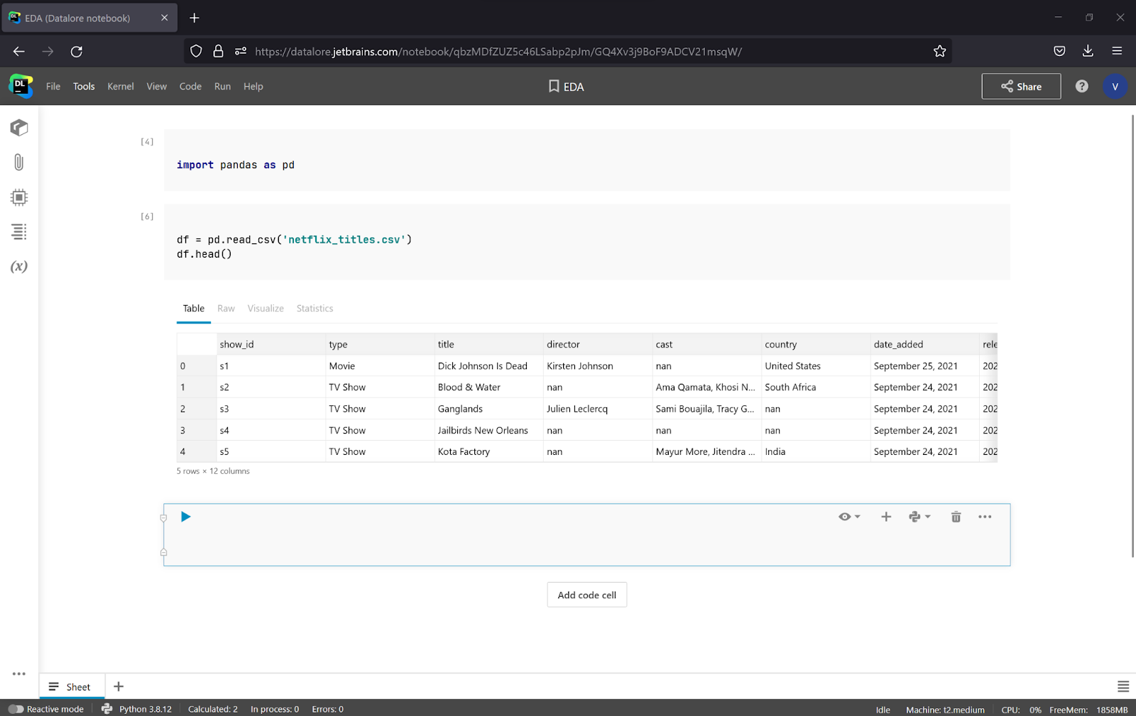
Starting work in Datalore is easy, as all of the necessary libraries are already installed. Just create a notebook and upload a dataset in Attached Data on the left-hand pane. To read a dataset with Pandas, let’s import it and read the CSV file with the code below:
import pandas as pd
df = pd.read_csv('netflix_titles.csv')
To observe the first five rows of the dataset, you can use a df.head()method.
Datalore lets you observe the data in a regular table, but that’s not all. You will also get all of the necessary dataset statistics of the dataset using the same method as df.info() and df.describe(), but in a more intuitive way. It is really handy, as you do not need to add any additional code. Let’s look at the statistics of the whole dataset.
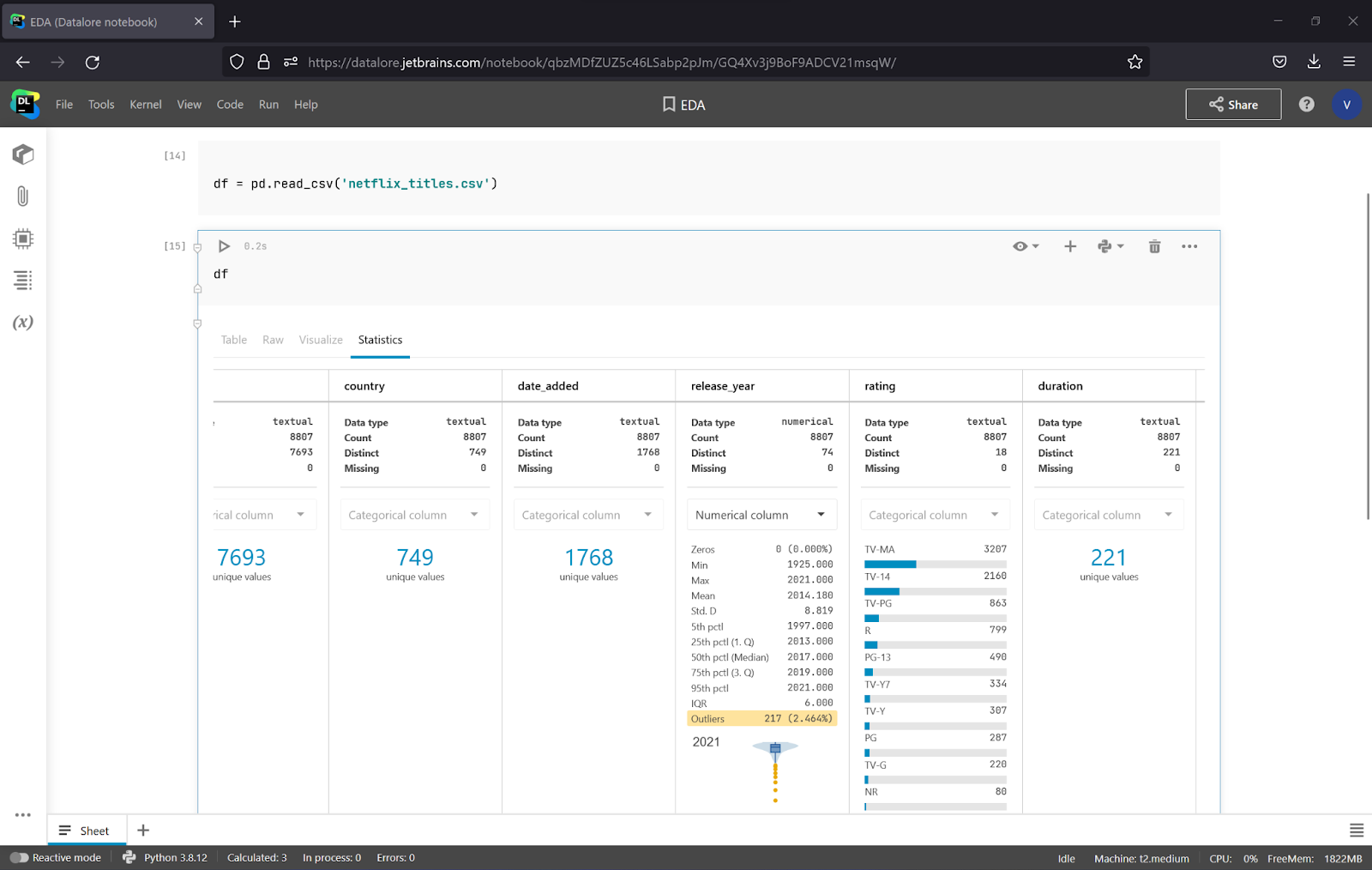
As you can see, there are 8807 rows. To get the number of features in addition to the number of instances, we can call df.shape and see that there are 12 features.
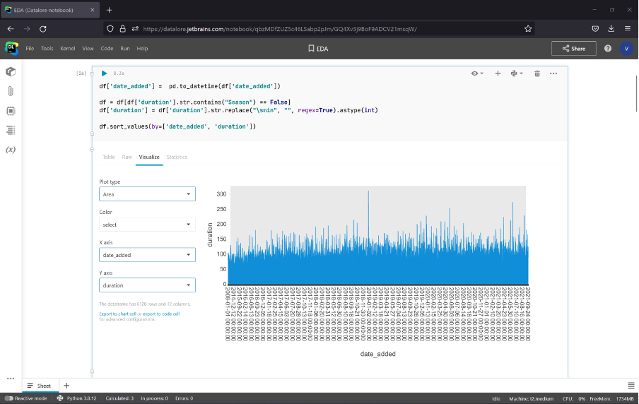
Datalore also lets you check your hypotheses quickly with a data visualization tool. Just click on the Visualize tab, choose the features for each axis, and plot the graph. Let’s see the correlation between a show’s duration and its release date.
First, we need to convert date_added to the DateTime format, remove duration rows, which correspond to seasons, and convert strings with min to int. It can be done with the following code.
df['date_added'] =  pd.to_datetime(df['date_added'])
df = df[df['duration'].str.contains("Season") == False]
df['duration'] = df['duration'].str.replace("\smin", "", regex=True).astype(int)
df.sort_values(by=['date_added', 'duration'])
Handling problems with data
You’ve likely noticed while observing the data that some values are NaN, which means there are missing values. This can negatively impact the accuracy of the analysis and decrease the performance of your machine learning model. Let’s see how we can handle this.
By using df.isnull().sum(), we can calculate the number of NaNs in each feature column.
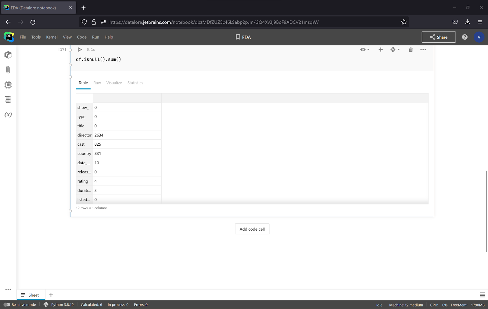
As shown above, there are a lot of missing values in the Director, Cast, and Country columns.
There are several possible approaches to handling missing values:
- Calculate the mean value of all occurrences and fill it in instead of the missing values. This is the most popular approach, but it adds a bias to the data distribution.
- Replace NaN values with the most frequent value of the feature. This can work well for categorical data.
- Drop rows with missing values. This approach lets the dataset keep “natural values,” but in the case of training a model, it can cause the generalization of problems. This is due to the lack of unique examples and the small overall number of training examples.
- Use machine learning algorithms such as K-NN or random forest to predict missing values. This can be the most accurate approach, but it is slow for big datasets.
For the Director, Cast, Country, and Rating columns, it could be a good idea to fill the missing data with the most frequent occurrences, as these features are categorical. To get the most frequent value in a director column, you can use the code below:
frequent_value = df[‘director’].value_counts().idxmax()
To replace the missing value in the column, use the code below:
df[‘director’] = df[‘director’].fillna(frequent_value)
As there are 4 columns to replace, let’s write a small chunk of code with a loop and observe the results.
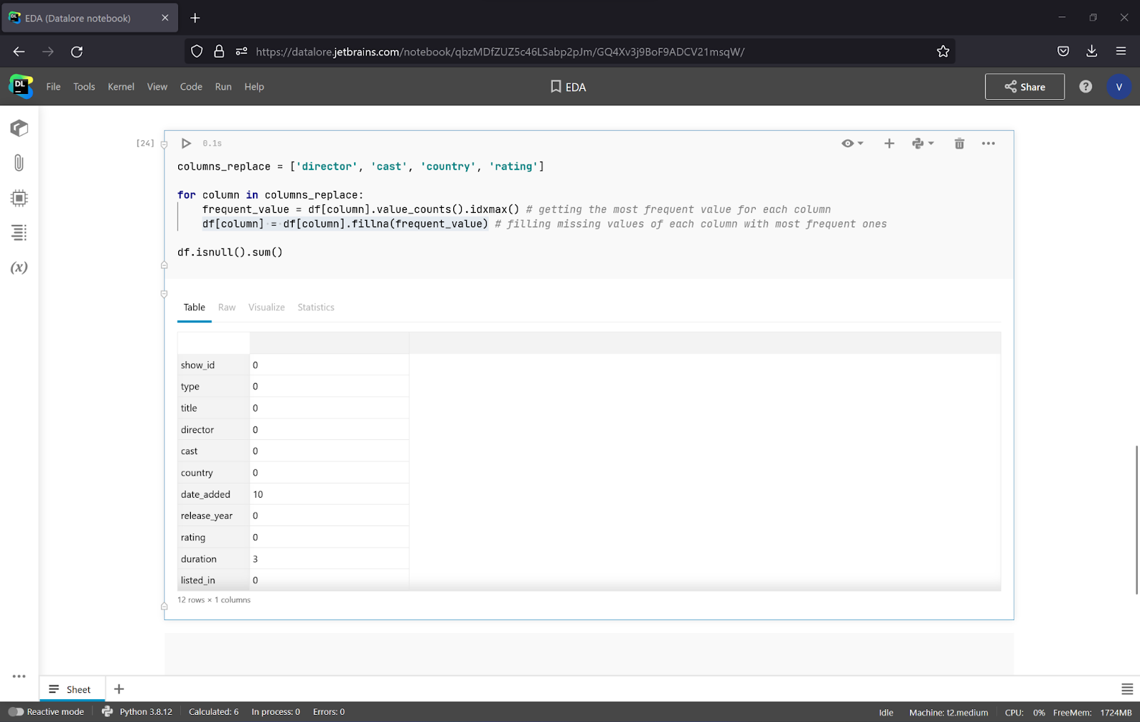
As you can see, all of the missing values of the 4 columns have disappeared. To deal with date_added and duration, let’s drop these columns, as it is difficult to fill in such data.
To drop the rows with missing values, use the code below:
df = df.dropna(axis = 0, how ='any')
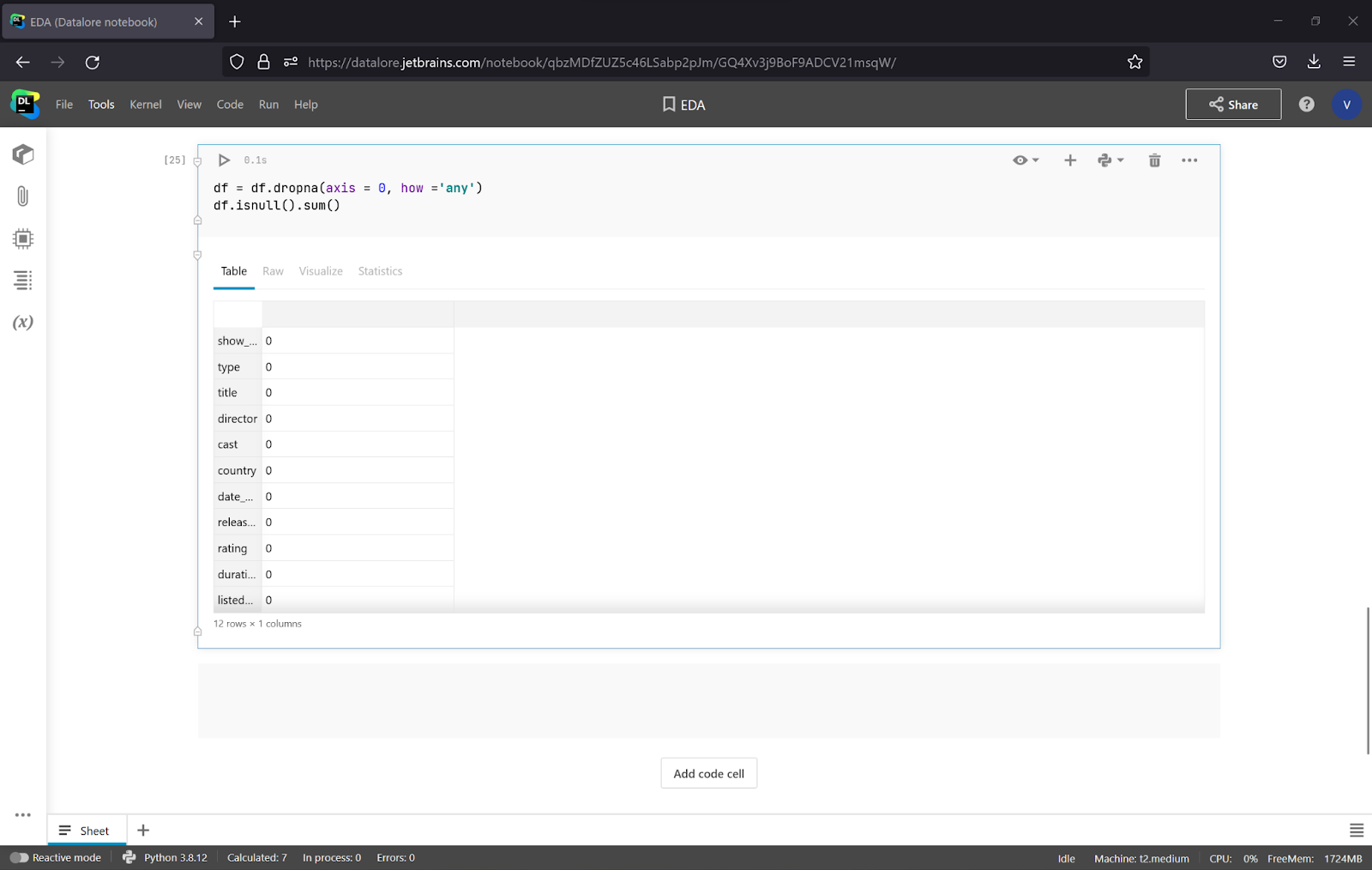
When you drop the rest of the missing values, you can see that there are no missing values anymore! You can try other approaches to handle missing values and get new insights.
Specific data visualization
As you’ve seen above, Datalore lets you visualize data in a handy way without any coding after uploading a dataset. You can use it to fulfill the majority of EDA needs. If you are not using Datalore or you need some specific plots (e.g. heatmaps), let’s look at how we can visualize our data with Plotly, a Python library that is widely used for exploratory data analysis.
Let’s draw a scatter matrix for the Type, Release_year, and Rating columns to get some insights. For that task, we will drop the rest of the columns and build a plot with the code below:
import plotly.graph_objects as go
import plotly.express as px
df_dropped = df.drop(columns=['show_id', 'title', 'director', 'cast', 'date_added', 'description', 'listed_in', 'duration', 'country'])
fig = px.scatter_matrix(df_dropped)
fig.show()
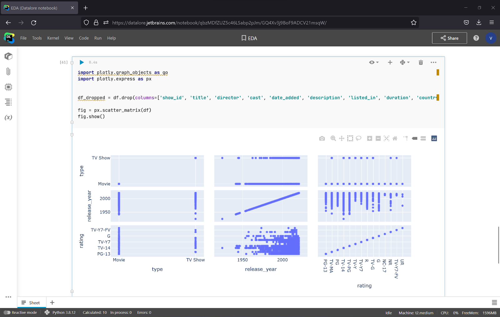
To make it more visual, it’s a good idea to specify the column that will be represented and apply coloring to the data.
fig = px.scatter_matrix(df_dropped,
    dimensions=["type", "release_year", "rating"],
    color="rating")
fig.show()
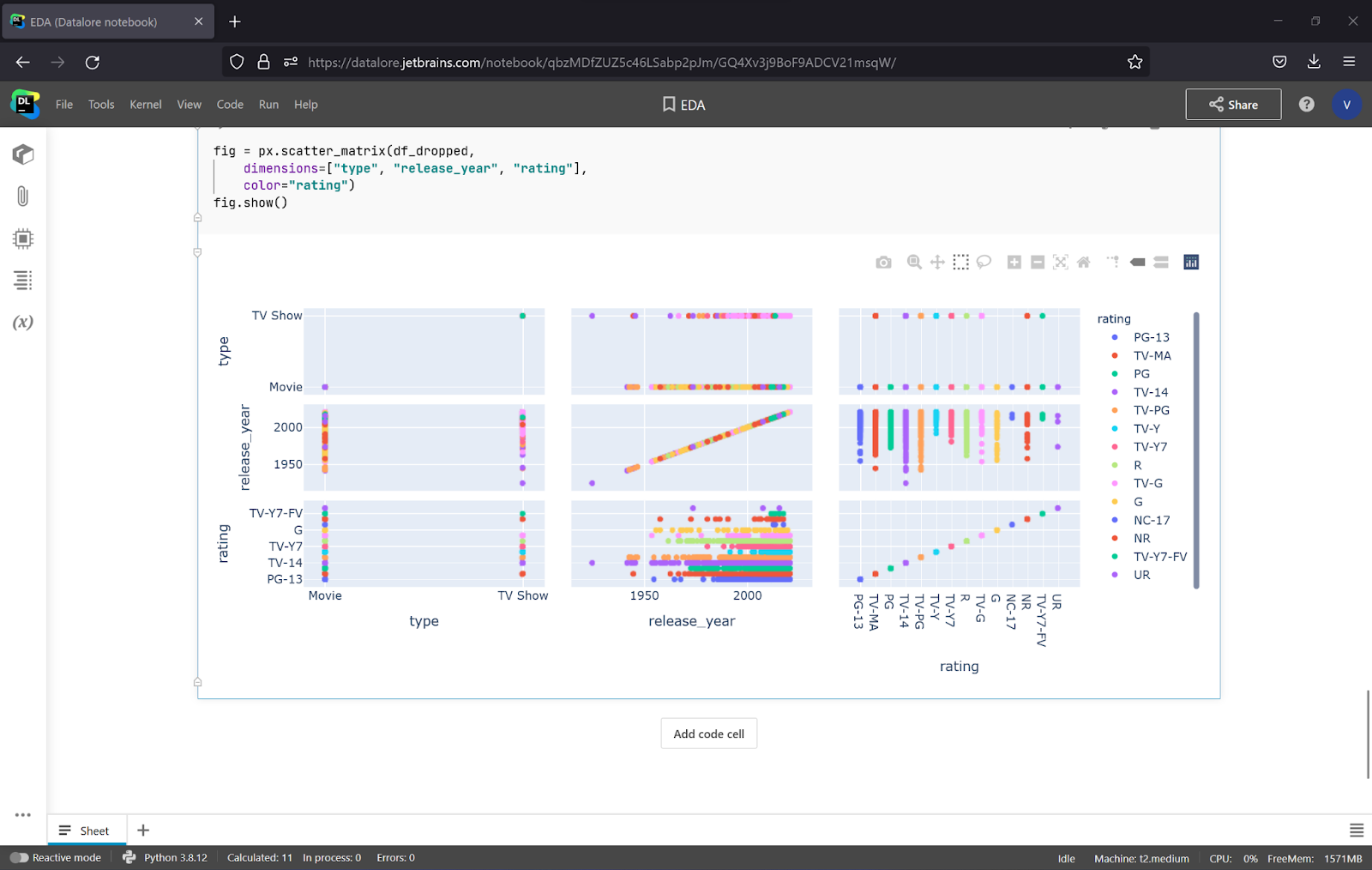
It looks like Netflix started using NC-17 and TV-Y7-FV ratings in the 2000s, and they only use the PG rating for movies. You can also check other correlations, but do not forget to transform duration and date_added to a standardized format (e.g. float and datetime). You can do so with the total_seconds()and to_datetime() methods.
To observe the connection between columns, you can use a density map. It will help you understand the degree of connection between values.
fig = px.density_heatmap(df, x=<strong>"release_year"</strong>, y=<strong>"type"</strong>)
fig.show()
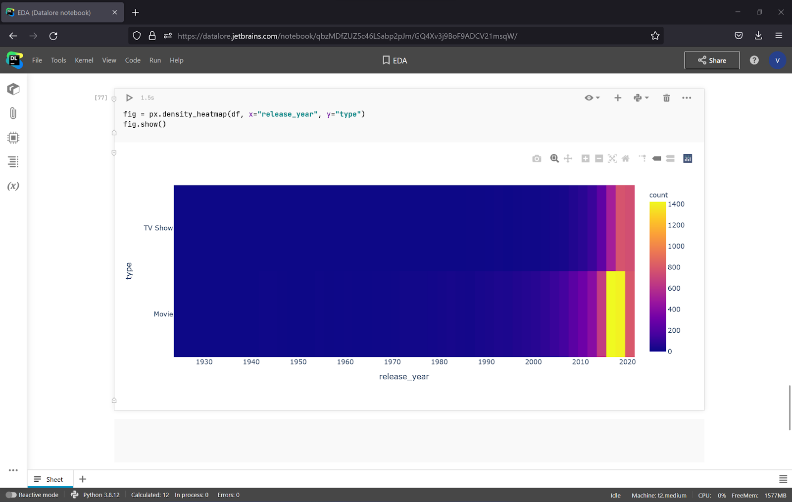
It looks like Netflix has been concentrating on movies in recent years. You can also try more options and compare more columns to get more insights.
Conclusion
Whether you want to make a decision based on data or train a machine learning model to make predictions, you need Exploratory Data Analysis. Python, Pandas, and Plotly are some of the must-have tools for this, as they make it easy and fast to explore data. To be more flexible and save even more time, you can also use Datalore, which provides you with a wide range of tools for Exploratory Data Analysis and the statistics and visualization tools needed to check your hypotheses.


