Datalore
Collaborative data science platform for teams
Risk Modeling in Python With Datalore and AI Assistant
This is a guest blog post by Ryan O’Connell, CFA, FRM.
Risk is an inherent part of the financial landscape, and as investors, we’re constantly seeking ways to quantify and mitigate it. By modeling risks, we can assess potential losses and make informed decisions. By quantifying risk, we can develop strategies to minimize risk exposure and optimize returns.
Python, with its rich ecosystem of libraries and tools, has become a go-to language for risk modeling. Its flexibility, scalability, and ease of use have made it a favorite among financial professionals. Furthermore, with Datalore AI, you can implement risk modeling techniques even as a non-professional data scientist. Datalore AI will help you generate Python code and fix any errors along the way.
In this article, we’ll explore a case study where we perform a Monte Carlo analysis for Value at Risk (VaR) on a stock portfolio, leveraging the power of Python, Datalore, and AI Assistant.
Disclaimer: This article is for informational and educational purposes only and is not intended to serve as personal financial advice.
If you have experience with Python, you can access the example Datalore notebook here. If you are new to Python, read on for a step-by-step walkthrough.
Why choose Python for risk modeling?
Python offers numerous benefits for financial professionals:
- An extensive ecosystem of libraries and tools for financial analysis and risk modeling:
- NumPy: A fundamental library for numerical computing, offering support for multi-dimensional arrays and mathematical functions.
- pandas: A powerful data manipulation and analysis library, providing data structures like DataFrames and Series for efficient handling of financial data.
- yfinance: A popular library for retrieving historical stock data from Yahoo Finance, enabling easy download and analysis of financial data.
- Python’s flexibility and scalability enable users to model a wide range of risk scenarios, from simple portfolios to complex financial instruments, and easily integrate with other tools and datasets.
- Easy to get started with, thanks to Datalore’s AI Assistant, which enhances the accessibility of risk modeling by providing intelligent code suggestions and error detection, allowing users to focus on high-level concepts.
For running intensive computations, such as the Monte Carlo simulation we will be implementing in this tutorial, Datalore offers access to powerful CPUs and GPUs.
Understanding risk modeling in Python
To start our risk modeling task, let’s first explore some key concepts and tools:
- Value at Risk (VaR): VaR quantifies the potential loss an investment or portfolio may incur over a given time horizon at a specific confidence level. It helps assess the risk associated with investments.
- Monte Carlo simulation: This computational technique relies on repeated random sampling to generate numerical results representing potential future outcomes. In risk modeling, it involves simulating numerous potential future scenarios based on assumed probability distributions (often using z-scores to represent deviations from the mean) to estimate the probability distribution of returns and assess risk.
The Monte Carlo simulation technique for VaR calculation involves the following steps:
- Define the portfolio and obtain historical price data.
- Calculate historical returns based on the price data.
- Estimate parameters of the return distribution (mean, standard deviation) from historical returns.
- Select your analysis parameters (number of simulations, VaR confidence level, time period, and initial portfolio size).
- Generate a large number of random scenarios for future returns using the estimated parameters.
- Calculate the corresponding portfolio value for each scenario.
- Sort the simulated portfolio values and determine the VaR at the desired confidence level.
- Repeating this process numerous times yields a distribution of potential portfolio values, allowing for risk assessment and data visualization.
In the following sections, we’ll walk through a practical example of implementing a Monte Carlo simulation for VaR calculation using Python, Datalore, and AI Assistant. We’ll leverage the power of Python libraries and Datalore’s intuitive interface to demonstrate how risk modeling can be made accessible to a wider audience.
Setting up the environment
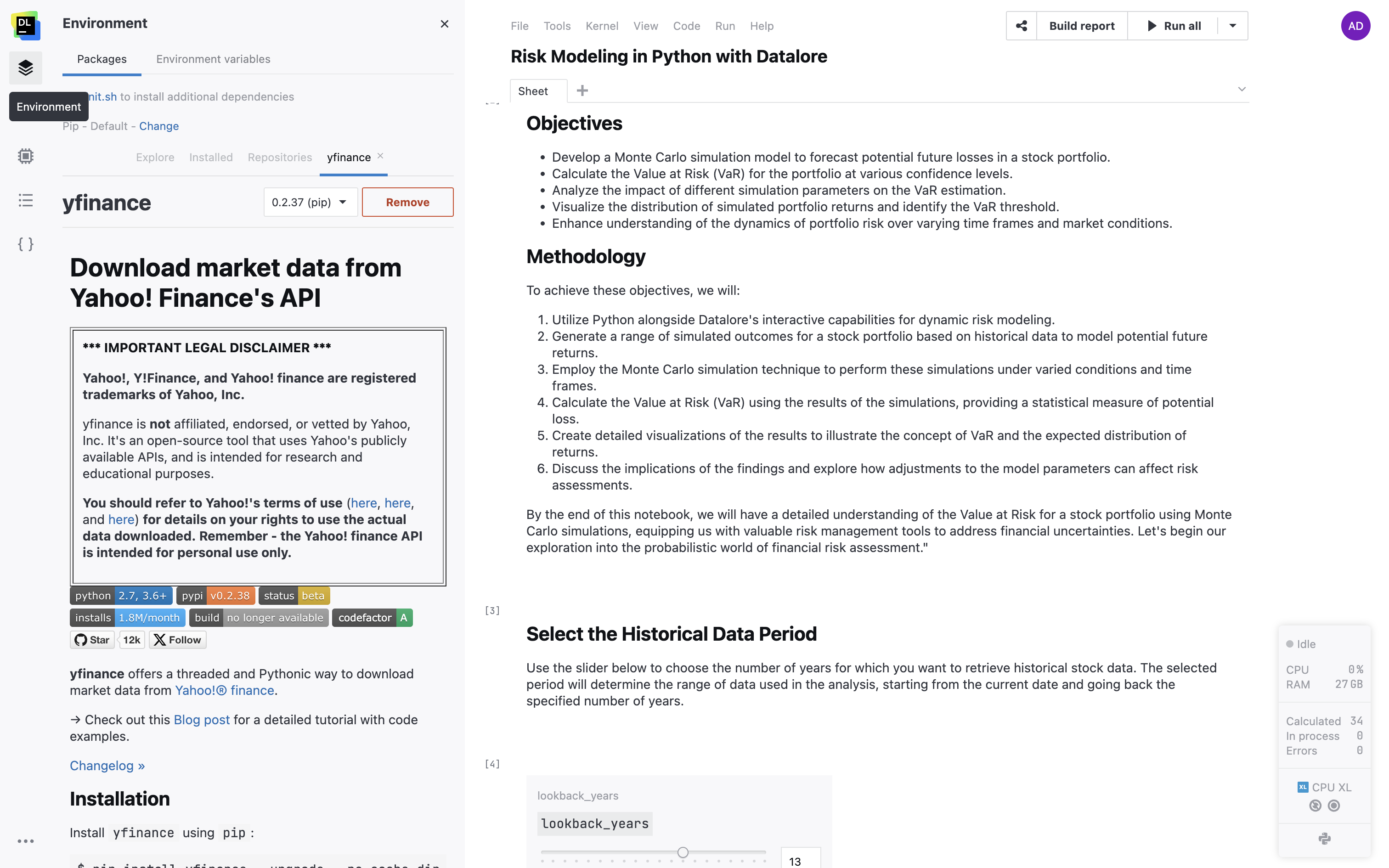
Before diving into the implementation, let’s set up our environment in Datalore. We’ll need to install the necessary libraries, such as yfinance, to retrieve historical stock data.
To install the required libraries, follow these steps:
- Open a new notebook in Datalore.
- Click on the Environment tab on the left sidebar.
- In the search bar, type “yfinance” and click on the Install button next to the package name.
Data retrieval and preprocessing
With our environment set up, let’s proceed with retrieving historical stock data using the yfinance library and preprocess it for our Monte Carlo simulation. Users can choose the stocks they want to include in the portfolio by providing a list of ticker symbols. This allows for personalized portfolio analysis based on individual preferences and investment strategies. A pre-selected list representing 15 diverse companies is currently available to choose from. A custom portfolio can be created as shown below:
We can also define the lookback period that we want to use for historical data as shown below:
We will base future return assumptions on this historical data, which is a common approach in financial modeling. However, it’s important to acknowledge that relying solely on historical data has its limitations, as past performance does not guarantee future results. Market conditions, economic cycles, and company-specific factors can change over time, making historical data less reliable for predicting future outcomes.
Furthermore, the choice of lookback period can introduce time selection bias, as the starting and ending dates of the historical data can significantly impact the results. For example, if the selected period captures a bull or bear market, it may not be representative of long-term market behavior.
We’ll use Datalore’s AI Assistant to guide us through the process of fetching data for a portfolio of stocks and performing the necessary data preprocessing steps. This includes calculating the daily returns for each stock, which will be a crucial input for our Monte Carlo simulation.
Daily returns provide a standardized measure of the price changes in our portfolio, allowing us to analyze the risk and potential outcomes of our investments. By leveraging the power of Datalore’s AI Assistant, we can efficiently retrieve historical data, handle missing values, and calculate returns, enabling us to focus on the high-level aspects of risk modeling.
| Prompt for AI |
| Write Python code that imports the necessary libraries (yfinance, pandas), accepts a list of user-selected stock tickers as input, fetches historical stock data for the specified tickers and time period using yfinance, concatenates the data into a single DataFrame, handles missing values by forward-filling, and calculates daily logarithmic returns for each stock. Assume that the user has already provided the list of stock tickers. |
The following code snippet was generated by Datalore’s AI Assistant:
import numpy as np
import yfinance as yf
import pandas as pd
from datetime import datetime, timedelta
import time

end = datetime.today().strftime('%Y-%m-%d')
start = (datetime.today() - timedelta(days=lookback_years*365)).strftime('%Y-%m-%d')

# Create an empty dictionary to store the data
data = {}

# Fetch historical data for each stock with a delay between requests
for ticker in tickers:
    data[ticker] = yf.download(ticker, start=start, end=end)
    time.sleep(1)  # Add a 1-second delay between each request

# Concatenate the data into a single DataFrame
portfolio_data = pd.concat([data[ticker]['Close'] for ticker in data.keys()], axis=1, keys=data.keys())

# Handle missing values by forward-filling
portfolio_data.fillna(method='ffill', inplace=True)

# Calculate daily log returns for each stock
daily_returns = np.log(portfolio_data / portfolio_data.shift(1))
daily_returns
Portfolio weighting
In this section, we’ll assign weights to each stock in our portfolio. Portfolio weights represent the proportion of each asset in the overall portfolio, which plays a crucial role in determining the portfolio’s risk and return characteristics. For this example, we will assume that the stocks are equally weighted (an equal amount of money is invested into each of them), but you can assign different weights to each stock based on your own portfolio. By carefully selecting the weights, investors can align their portfolios with their risk preferences and investment objectives.
| Prompt for AI |
| Please write a Python code snippet that calculates equal weights for each stock in the portfolio using the ‘tickers’ list defined earlier. Store the weights in a dictionary called ‘weights’, where the keys are the stock tickers and the values are the corresponding weights. Ensure that the sum of the weights equals 1. |
The following code was generated by Datalore’s AI Assistant:
# Define the number of stocks in the portfolio
num_stocks = len(tickers)
# Calculate equal weights for each stock and store in a dictionary
weights = {ticker: 1.0/num_stocks for ticker in tickers}
# Print weights to verify that the sum equals 1
print(weights)
print("Sum of weights: ", sum(weights.values()))
Portfolio annualized returns and expected returns
To assess the potential returns of our portfolio, we’ll calculate the annualized returns and expected returns based on the historical data. Annualized returns provide a standardized measure of the average yearly returns, allowing for comparisons across different time periods. Expected returns, derived from historical data, serve as an estimate of future returns, which is a key input for the Monte Carlo simulation.
| Prompt for AI |
| Please provide a Python code snippet that calculates the annualized returns and expected returns for each stock in the portfolio using the ‘daily_returns’ DataFrame. Assume 252 trading days in a year. Then, calculate the portfolio’s annualized returns and expected returns using the ‘weights’ dictionary defined earlier. |
Datalore AI Assistant generates the following code:
# Calculate daily log returns for each stock
daily_returns = np.log(portfolio_data / portfolio_data.shift(1))

# Calculate the mean daily log return for each stock
mean_daily_returns = daily_returns.mean()

# Annualize the log returns
annualized_returns = mean_daily_returns * 252

# Consider the expected returns to be the same as annualized returns
expected_returns = annualized_returns

# Print the annualized and expected returns
print("Annualized Returns: ", annualized_returns)
print("Expected Returns: ", expected_returns)

# Create a dataframe for the weights from the weights dictionary
weights_df = pd.DataFrame(list(weights.values()), index=weights.keys(), columns=['weight'])

# Calculate the portfolio's annualized return
portfolio_annualized_return = weights_df['weight'].dot(annualized_returns)

# Calculate the portfolio's expected return
portfolio_expected_return = weights_df['weight'].dot(expected_returns)

# Print portfolio's annualized and expected return
print("Portfolio's Annualized Return: ", portfolio_annualized_return)
print("Portfolio's Expected Return: ", portfolio_expected_return)
Portfolio standard deviation and covariance matrix
To quantify the risk of our portfolio, we’ll calculate the annualized portfolio standard deviation using a covariance matrix. A covariance matrix captures the relationships between the returns of different stocks in the portfolio, providing a measure of how they move together. By incorporating a covariance matrix, we can account for the diversification effects and assess the overall portfolio risk.
| Prompt for AI |
| Please provide a Python code snippet that calculates the annualized covariance matrix using the ‘daily_returns’ DataFrame. Then, calculate the annualized portfolio standard deviation using the covariance matrix and the ‘weights’ dictionary. Assume 252 trading days in a year. |
Datalore AI Assistant generates the following code:
# Import additional necessary libraries
import numpy as np
# Calculate the covariance matrix of daily returns
cov_matrix = daily_returns.cov()
# Annualize the covariance matrix
annualized_cov_matrix = cov_matrix * 252
# Print the annualized covariance matrix
print("Annualized Covariance Matrix: \n", annualized_cov_matrix)
# Calculate the portfolio standard deviation
portfolio_std_dev = np.sqrt(np.dot(weights_df['weight'].T, np.dot(annualized_cov_matrix, weights_df['weight'])))
# Print the portfolio standard deviation
print("Portfolio's Annualized Standard Deviation: ", portfolio_std_dev)
Select simulation parameters
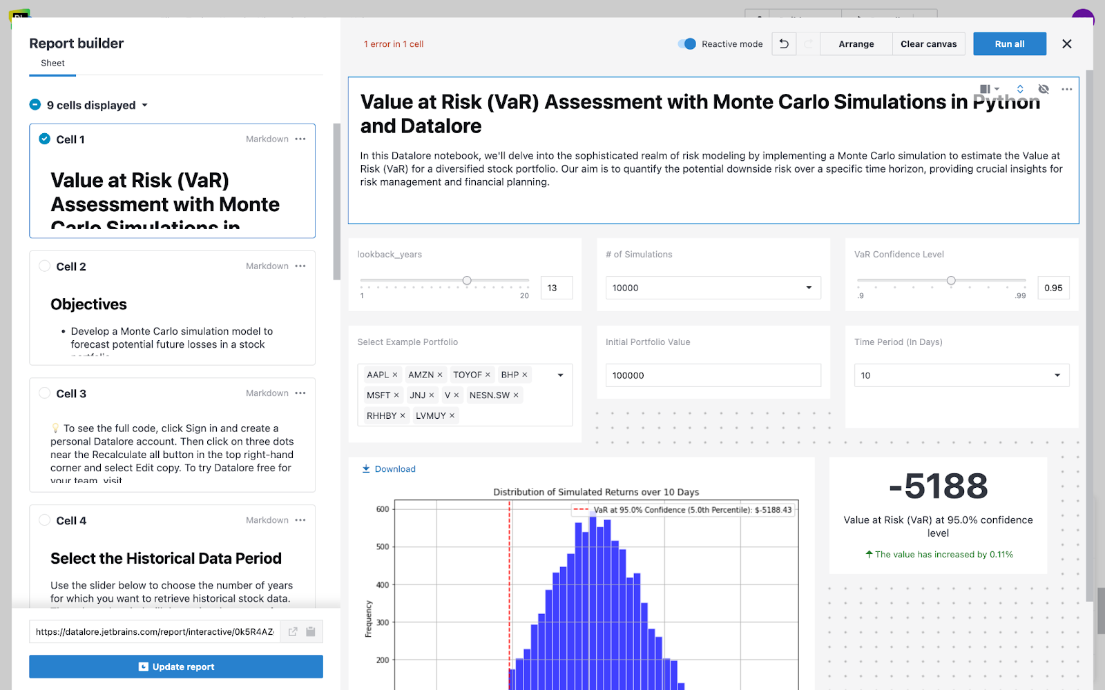
The Monte Carlo simulation for the Value at Risk (VaR) calculation relies on several key parameters that users can customize to align with their specific requirements and risk assessment needs. These parameters include the number of simulations, VaR confidence level, time period, and initial portfolio value.
- Number of simulations: Use the dropdown menu to choose the number of simulations you want to run for the Monte Carlo analysis. A higher number of simulations may provide more accurate results by generating a larger sample size of potential outcomes. However, increasing the number of simulations also requires more computing power and time to complete the analysis. Datalore offers multiple CPU and GPU machines, so you can speed up the computation process by selecting a more powerful option.
- VaR confidence level: The VaR confidence level determines the probability that the actual loss will not exceed the calculated VaR. Adjust the slider to select the desired confidence level for the VaR calculation. Common confidence levels include 95% and 99%. A higher confidence level indicates a more conservative risk assessment, as it captures a larger portion of the potential loss distribution.
- Time period: The time period defines the holding period for which the potential loss is estimated. Choose the time period for the VaR calculation from the dropdown menu. The available options represent different holding periods, such as 1 day (one-day VaR), 10 days (two-week VaR), 21 days (one-month VaR), or 252 days (one-year VaR). The selected time period should align with your investment horizon and risk management objectives. Shorter time periods are suitable for short-term risk assessment, while longer periods are more appropriate for strategic planning.
- Initial portfolio value: Enter the initial value of your portfolio in the provided input field. This value represents the total amount of capital invested across all assets in the portfolio. Setting the initial portfolio value allows you to assess the potential dollar value of losses based on the calculated VaR percentage. It helps in translating the relative risk measure (VaR percentage) into an absolute dollar amount.
The Monte Carlo simulation, powered by the user-defined parameters, generates a large number of random scenarios based on the historical data and calculates the portfolio value for each scenario. The VaR is then determined by identifying the loss threshold at the specified confidence level, providing investors with a quantitative measure of the potential downside risk.
Defining functions for Monte Carlo simulation
Monte Carlo simulation is a powerful technique for modeling the probability of different outcomes in a process that cannot easily be predicted due to the intervention of random variables. In our case, we’ll define a function that performs a Monte Carlo simulation to generate a large number of potential future return scenarios for our portfolio.
| Prompt for AI |
| Define a Monte Carlo simulation function that takes the portfolio’s expected return, standard deviation, number of simulations, and number of trading days as input parameters. The function should generate random numbers from a standard normal distribution, convert them into daily returns using the portfolio’s expected return and standard deviation, and return the daily returns. |
Datalore AI Assistant generates the following code:
# Define the Monte Carlo simulation function
def monte_carlo_simulation(expected_return, std_dev, num_simulations, num_trading_days):
    # Generate random samples from a normal distribution for return deviations
    rand_returns = np.random.normal(0, 1, (num_simulations, num_trading_days))
    # Calculate simulated returns by adjusting expected returns and adding scaled random deviations
    period_returns = (1 + expected_return) ** (num_trading_days / 252) - 1 + std_dev * rand_returns * np.sqrt(num_trading_days / 252)
    # Return the array of simulated returns for each trading day and simulation
    return period_returns
Running Monte Carlo simulations
Now that we have defined the Monte Carlo simulation function, let’s run the simulations to generate potential future return scenarios for our portfolio.
| Prompt for AI |
| Write Python code that runs the Monte Carlo simulation function with a reasonable number of simulations and trading days, using the portfolio’s expected return and standard deviation calculated earlier. Store the results in a variable for further analysis. |
Datalore AI Assistant generates the following code:
# Run the Monte Carlo simulation
simulated_daily_returns = monte_carlo_simulation(portfolio_expected_return, portfolio_std_dev, number_of_simulations, time_period)
Calculating Value at Risk (VaR)
Value at Risk (VaR) is a widely used risk metric that quantifies the potential loss that a portfolio may incur over a specific time horizon, given a certain level of confidence. By calculating VaR based on the simulated returns from our Monte Carlo simulation, we can assess the downside risk of our portfolio and make informed risk management decisions.
| Prompt for AI |
| Write Python code that calculates the Value at Risk (VaR) of our portfolio based on the simulated returns. Use the defined initial investment. Calculate the portfolio values on the last trading day using the simulated daily returns. Calculate the VaR at the selected confidence level by determining the corresponding percentile of the simulated portfolio returns on the last trading day. Express the VaR in dollar terms. |
Datalore AI Assistant generates the following code:
# Calculate the portfolio values at the end of the period
portfolio_values_end_period = initial_investment * (1 + simulated_period_returns)

# VaR Confidence Level declaration
percentile_level = 100 - (VaR_confidence_level*100)

# Calculate VaR at the specified confidence level
VaR = np.percentile(portfolio_values_end_period, percentile_level) - initial_investment
print(f"Value at Risk (VaR) at {VaR_confidence_level*100}% confidence level is: $", VaR)
Visualizing Value at Risk (VaR) on a distribution plot
To better understand the concept of Value at Risk (VaR) and how it relates to the distribution of simulated portfolio returns, let’s create a visual representation. By plotting the distribution of simulated returns on the last trading day and marking the VaR on the left tail of the distribution, we can gain a clearer picture of the potential downside risk.
| Prompt for AI |
| Write Python code that visualizes the Value at Risk on a distribution plot of the simulated daily portfolio gains and losses. Calculate the portfolio values at the end of the simulation period by multiplying the initial investment with the simulated cumulative returns on the last trading day. Then, subtract the initial investment from the portfolio values to get the dollar gains and losses. Create a histogram of these gains and losses using pyplot, which should resemble a bell curve showing both positive and negative values. Use the Value at Risk value calculated earlier in the code. Add a vertical line on the plot to indicate the position of the VaR on the left tail of the distribution. Include appropriate labels for the x-axis (Portfolio Gains/Losses ($)), y-axis (Frequency), and a title for the plot (Distribution of Simulated Portfolio Gains and Losses). Also, add a legend to the plot displaying the VaR confidence level and percentile. |
Datalore AI Assistant generates the following code:
import matplotlib.pyplot as plt
import numpy as np

# Calculate the period dollar returns at the end of the 10-day period for each simulation
period_dollar_returns = portfolio_values_end_period[:, -1] - initial_investment

# Create the histogram plot using Matplotlib with blue bars and white outlines
plt.figure(figsize=(10, 6))
plt.hist(period_dollar_returns, bins=50, color='blue', edgecolor='white', alpha=0.75)

# Add the VaR line
plt.axvline(x=VaR, color='red', linestyle='--', linewidth=1.5,
            label=f'VaR at {VaR_confidence_level*100}% Confidence ({percentile_level}th Percentile): ${VaR:.2f}')

# Set the plot title and labels
plt.title(f'Distribution of Simulated Returns over {time_period} Days')
plt.xlabel('Portfolio Gains/Losses ($)')
plt.ylabel('Frequency')
# Add a legend
plt.legend()
# Add grid lines
plt.grid(True)
# Show the plot
plt.show()
Analyzing the distribution of simulated portfolio gains and losses
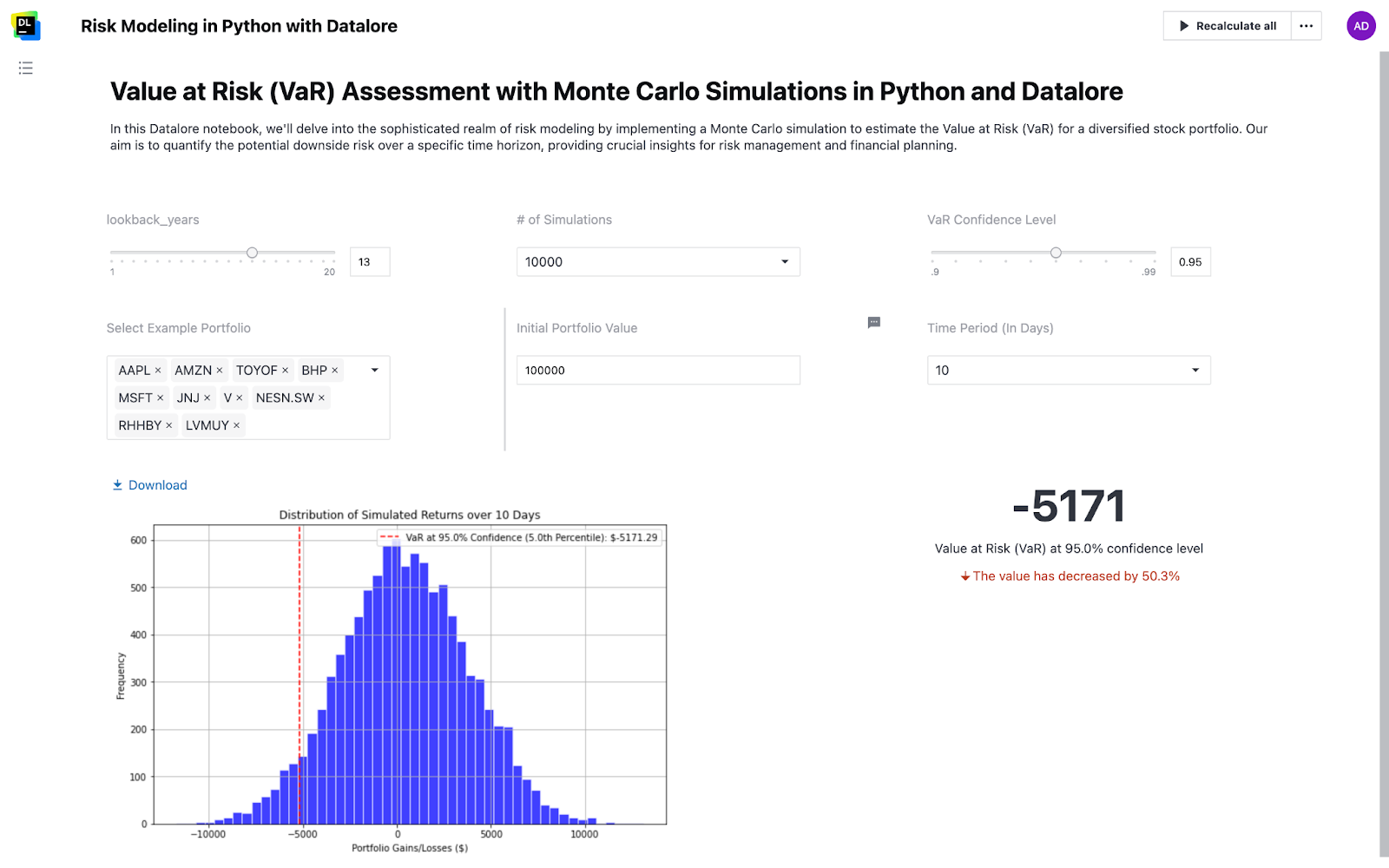
The histogram below visualizes the distribution of simulated daily portfolio gains and losses obtained from the Monte Carlo simulation. It provides valuable insights into the potential outcomes and helps us understand the risk profile of our portfolio.
The scenario to generate this visualization included the following parameters:
- Number of Simulations: 10,000
- Time Period: 10 Days
- Confidence Level: 95%
- Initial Investment: $100,000
You can see the returns in dollar values of the 10,000 simulations below:
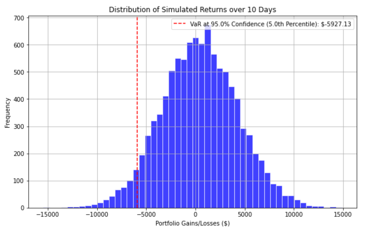
The x-axis represents the daily gains and losses in dollar terms, while the y-axis shows the frequency of occurrence for each bin. The histogram typically resembles a bell curve, with both positive and negative values distributed around the central peak.
The vertical red dashed line on the left side of the distribution indicates the Value at Risk (VaR) at the specified confidence level and percentile. In this example, the VaR is calculated at a 95% confidence level, which corresponds to the fifth percentile of the simulated portfolio values on the last trading day. If we lined up all of the simulated portfolio values from lowest to highest, the 5th percentile would be the value separating the bottom 5% from the rest. This value corresponds to the VaR at the 95% confidence level, representing the maximum potential loss expected to be exceeded only 5% of the time.
The VaR line serves as a visual representation of the potential downside risk. It signifies the maximum loss that the portfolio could incur over the specified time period, with a probability equal to the chosen confidence level. For instance, if the VaR at a 95% confidence level is $5,927.13, it means that there is a 95% probability that the portfolio will not lose more than $5,927.13 over the 10-day time horizon.
By examining the histogram and the position of the VaR line, investors can assess the risk profile of their portfolio and make informed decisions based on their risk tolerance. A longer left tail of the distribution indicates a higher potential for extreme losses, while a shorter left tail suggests a more conservative risk profile.
It’s important to note that the VaR calculation is based on historical data and assumes that future returns will follow a similar distribution. However, market conditions can change, and extreme events not captured in the historical data may occur. Therefore, investors should use VaR as one of the many tools in their risk management arsenal and combine it with other risk measures and qualitative analysis.
Conclusion
In this tutorial, you’ve learned how to implement Monte Carlo simulations and Value at Risk (VaR) analyses to assess potential losses in stock portfolios with Python and Datalore. We’ve discussed important assumptions, potential algorithm limitations, and biases, as well as important parameters of risk assessment, such as the number of simulations, the confidence level for VaR, and the investment period.
For hands-on experience and a deeper understanding of the risk model, engage with a notebook and associated interactive Datalore report to customize simulations as per your requirements.