Analyzing Data in Amazon Redshift with Pandas

Redshift is Amazon Web Services’ data warehousing solution. They’ve extended PostgreSQL to better suit large datasets used for analysis. When you hear about this kind of technology as a Python developer, it just makes sense to then unleash Pandas on it. So let’s have a look to see how we can analyze data in Redshift using a Pandas script!
Setting up Redshift
If you haven’t used Redshift before, you should be able to get the cluster up for free for 2 months. As long as you make sure that you don’t use more than 1 instance, and you use the smallest available instance.
To play around, let’s use Amazon’s example dataset, and to keep things very simple, let’s only load the ‘users’ table. Configuring AWS is a complex subject, and they’re a lot better at explaining how to do it than we are, so please complete the first four steps of the AWS tutorial for setting up an example Redshift environment. We’ll use PyCharm Professional Edition as the SQL client.
Connecting to Redshift
After spinning up Redshift, you can connect PyCharm Professional to it by heading over to the database tool window (View | Tool Windows | Database), then use the green ‘+’ button, and select Redshift as the data source type. Then fill in the information for your instance:
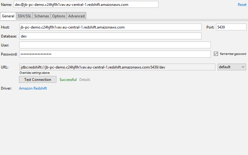
Make sure that when you click the ‘test connection’ button you get a ‘connection successful’ notification. If you don’t, make sure that you’ve correctly configured your Redshift cluster’s VPC to allow connections from 0.0.0.0/0 on port 5439.
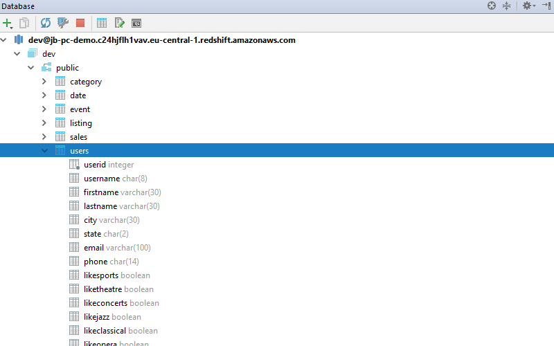
Now that we’ve connected PyCharm to the Redshift cluster, we can create the tables for Amazon’s example data. Copy the first code listing from here, and paste it into the SQL console that was opened in PyCharm when you connected to the database. Then execute it by pressing Ctrl + Enter, when PyCharm asks which query to execute, make sure to select the full listing. Afterward, you should see all the tables in the database tool window:
To load the sample data, go back to the query window, and use the Redshift ‘load’ command to load data from an Amazon S3 bucket into the database:
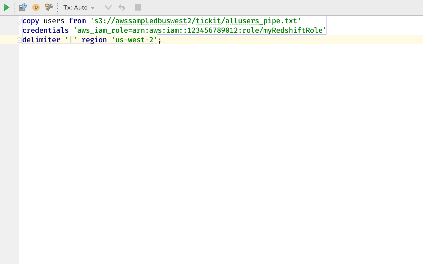
The IAM role identifier should be the identifier for the IAM role you’ve created for your Redshift cluster in the second step in the Amazon tutorial. If everything goes right, you should have about 50,000 rows of data in your users table after the command completes.
Loading Redshift Data into a Pandas Dataframe
So let’s get started with the Python code! In our example we’ll use Pandas, Matplotlib, and Seaborn. The easiest way to get all of these installed is by using Anaconda, get the Python 3 version from their website. After installing, we need to choose Anaconda as our project interpreter:
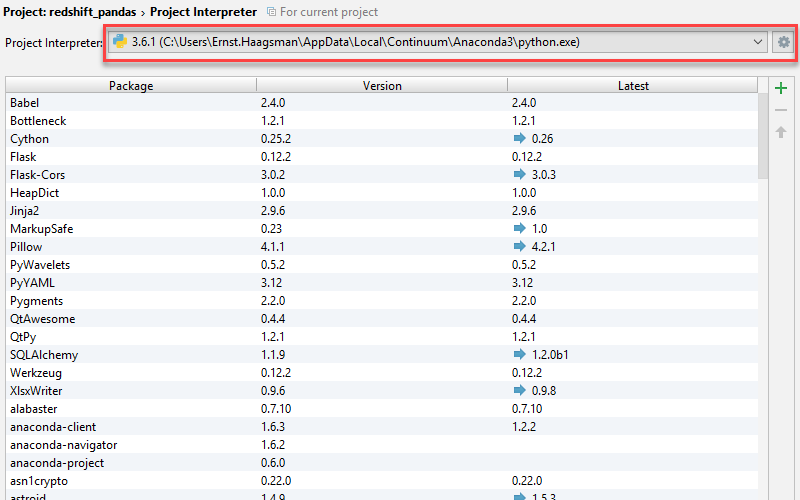
If you can’t find Anaconda in the dropdown, you can click the settings “gear” button, and then select ‘Add Local’ and find your Anaconda installation on your disk. We’re using the root Anaconda environment without Conda, as we will depend on several scientific libraries which are complicated to correctly install in Conda environments.
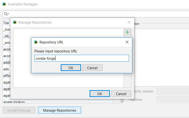
Pandas relies on SQLAlchemy to load data from an SQL data source. So let’s use the PyCharm package manager to install sqlalchemy: use the green ‘+’ button next to the package list and find the package. To make SQLAlchemy work well with Redshift, we’ll need to install both the postgres driver, and the Redshift additions. For postgres, you can use the PyCharm package manager to install psycopg2. Then we need to install sqlalchemy-redshift to teach SQLAlchemy the specifics of working with a Redshift cluster. This package is unfortunately not available in the default Anaconda repository, so we’ll need to add a custom repository.
To add a custom repository click the ‘Manage Repositories’ button, and then use the green ‘+’ icon to add the ‘conda-forge’ channel. Afterwards, close the ‘Manage Repositories’ screen, and install sqlalchemy-redshift. Now that we’ve done that, we can start coding!
To show how it’s done, let’s analyze something simple in Amazon’s dataset, the users dataset holds fictional users, and then indicates for every user if they like certain types of entertainment. Let’s see if there’s any correlation between the types of entertainment.
As always, the full code is available on GitHub.
Let’s open a new Python file, and start our analysis. At first, we need to load our data. Redshift is accessed just like a regular PostgreSQL database, just with a slightly different connection string to use the redshift driver:
connstr = 'redshift+psycopg2://<username>:<password>@<your cluster>.redshift.amazonaws.com:5439/<database name>'
Also note that Redshift by default listens on port 5439, rather than Postgres’ 5432.
After we’ve connected we can use Pandas’ standard way to load data from an SQL database:
import pandas as pd
from sqlalchemy import create_engine

engine = create_engine(connstr)

with engine.connect() as conn, conn.begin():
   df = pd.read_sql("""
           select
             likesports as sports,
             liketheatre as theater,
             likeconcerts as concerts,
             likejazz as jazz,
             likeclassical as classical,
             likeopera as opera,
             likerock as rock,
             likevegas as vegas,
             likebroadway as broadway,
             likemusicals as musicals
           from users;""", conn)
The dataset holds users’ preferences as False, None, or True. Let’s interpret this as True being a ‘like’, None being ambivalent, and False being a dislike. To make a correlation possible, we should convert this into numeric values:
# Map dataframe to have 1 for 'True', 0 for null, and -1 for False
def bool_to_numeric(x):
   if x:
       return 1
   elif x is None:
       return 0
   else:
       return -1

df = df.applymap(bool_to_numeric)
And now we’re ready to calculate the correlation matrix, and present it. To present it we’ll use Seaborn’s heatmap. We’ll also create a mask to only show the bottom half of the correlation matrix (the top half mirrors the bottom).
import seaborn as sns
import matplotlib.pyplot as plt
import numpy as np

# Calculate correlations
corr = df.corr()

mask = np.zeros_like(corr)
mask[np.triu_indices_from(mask)] = True

sns.heatmap(corr,
           mask=mask,
           xticklabels=corr.columns.values,
           yticklabels=corr.columns.values)

plt.xticks(rotation=45)
plt.yticks(rotation=45)

plt.tight_layout()
plt.show()
After running this code, we can see that there are no correlations in the dataset:
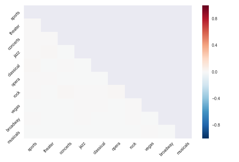
Which is strong evidence for Amazon’s sample dataset being a sample dataset. QED.
Fortunately, PyCharm also works great with real datasets in Redshift. Let us know in the comments what data you’re interested in analyzing!

Subscribe to PyCharm Blog updates