Anomaly Detection in Machine Learning Using Python

In recent years, many of our applications have been driven by the high volume of data that we are able to collect and process. Some may refer to us being in the age of data. One of the essential aspects of handling such a large amount of data is anomaly detection – processes that enable us to identify outliers, data that is outside the bounds of expectation and demonstrate behavior that is out of the norm. In scientific research, anomaly data points could be a cause of technical issues and may need to be discarded when drawing conclusions, or it could lead to new discoveries.
In this blog post, we’ll see why using machine learning for anomaly detection is helpful and explore key techniques for detecting anomalies using Python. You’ll learn how to implement popular methods like OneClassSVM and Isolation Forest, see examples of how to visualize these results and understand how to apply them to real-world problems.
Where is anomaly detection used?
Anomaly detection has also been a crucial part of modern-day business intelligence, as it provides insights into what could possibly go wrong and may also identify potential problems. Here are some examples of using anomaly detection in modern-day business.
Security alerts
There are some cyber security attacks that can be detected via anomaly detection; for example, a spike in request volume may indicate a DDoS attack, while suspicious login behavior, like multiple failing attempts, may indicate unauthorized access. Detecting suspicious user behavior may indicate potential cyber security threats, and companies can act on them accordingly to prevent or minimize the damage.
Fraud detection
In financial organizations, for example, banks can use anomaly detection to highlight suspicious account activities, which may be an indication of illegal activities like money laundering or identity theft. Suspicious transactions can also be a sign of credit card fraud.
Observability
One of the common practices for web services is to collect metrics of the real-time performance of the service if there is abnormal behavior in the system. For example, a spike in memory usage may show that something in the system isn’t functioning properly, and engineers may need to address it immediately to avoid a break in service.
Why use machine learning for anomaly detection?
Although traditional statistical methods can also help find outliers, the use of machine learning for anomaly detection has been a game changer. With machine learning algorithms, more complex data (e.g. with multiple parameters) can be analyzed all at once. Machine learning techniques also provide a means to analyze categorical data that isn’t easy to analyze using traditional statistical methods, which are more suited to numerical data.
A lot of time, these anomaly detection algorithms are programmed and can be deployed as an application (see our FastAPI for Machine Learning tutorial) and run as requested or at scheduled intervals to detect any anomalies. This means that they can prompt immediate actions within the company and can also be used as reporting tools for business intelligence teams to review and adjust strategies.
Types of anomaly detection techniques and algorithms
There are generally two main types of anomaly detection: outlier detection and novelty detection.
Outlier detection
Outlier detection is sometimes referred to as unsupervised anomaly detection, as it is assumed that in the training data, there are some undetected anomalies (thus unlabeled), and the approach is to use unsupervised machine learning algorithms to pick them out. Some of these algorithms include one-class support vector machines (SVMs), Isolation Forest, Local Outlier Factor, and Elliptic Envelope.
Novelty detection
On the other hand, novelty detection is sometimes referred to as semi-supervised anomaly detection. Since we assume that all training data doesn’t solely consist of anomalies, they’re all labeled as normal. The goal is to detect whether or not new data is an anomaly, which is sometimes referred to as a novelty. The algorithms used in outlier detection can also be used for novelty detection, provided that there are no anomalies in the training data.
Other than the outlier detection and novelty detection mentioned, it is also very common to require anomaly detection in time series data. However, since the approach and technique used for time series data are often different from the algorithms mentioned above, we’ll discuss these in detail at a later date.
Code example: finding anomalies in the Beehives dataset
In this blog post, we’ll be using this Beehives dataset as an example to detect any anomalies in the hives. This data set provides various measurements of the hive (including the temperature and relative humidity of the hive) at various times.
Here, we’ll be showing two very different methods for discovering anomalies. They are OneClassSVM, which is based on support vector machine technology, which we’ll use for drawing decision boundaries, and Isolation Forest, which is an ensemble method similar to Random Forest.
Example: OneClassSVM
In this first example, we’ll be using the data of hive 17, assuming bees will keep their hive in a constant pleasant environment for the colony; we can look at whether this is true and if there are times that the hive experiences anomaly temperature and relative humidity levels. We’ll use OneClassSVM to fit our data and look at the decision-making boundaries on a scatter plot.
The SVM in OneClassSVM stands for support vector machine, which is a popular machine learning algorithm for classification and regressions. While support vector machines can be used to classify data points in high dimensions, by choosing a kernel and a scalar parameter to define a frontier, we can create a decision boundary that includes most of the data points (normal data), while retaining a small number of anomalies outside of the boundaries to represent the probability (nu) of finding a new anomaly. The method of using support vector machines for anomaly detection is covered in a paper by Scholkopf et al. entitled Estimating the Support of a High-Dimensional Distribution.
1. Start a Jupyter project
When starting a new project in PyCharm (Professional 2024.2.2), select Jupyter under Python.
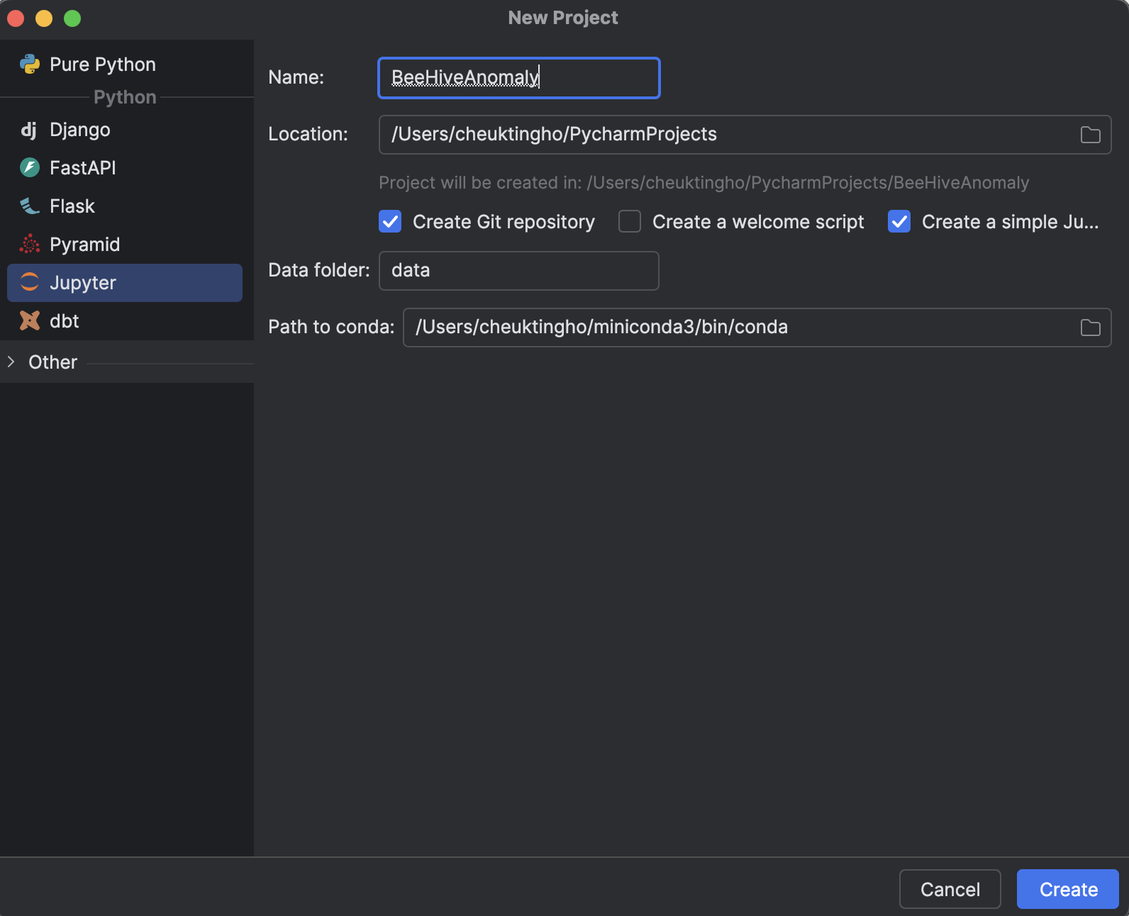
The benefit of using a Jupyter project (previously also known as a Scientific project) in PyCharm is that a file structure is generated for you, including a folder for storing your data and a folder to store all the Jupyter notebooks so you can keep all your experiments in one place.
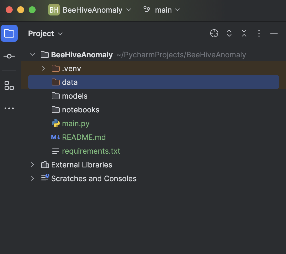
Another huge benefit is that we can render graphs very easily with Matplotlib. You will see that in the steps below.
2. Install dependencies
Download this requirements.txt from the relevant GitHub repo. Once you place it in the project directory and open it in PyCharm, you will see a prompt asking you to install the missing libraries.

Click on Install requirements, and all of the requirements will be installed for you. In this project, we’re using Python 3.11.1.
3. Import and inspect the data
You can either download the “Beehives” dataset from Kaggle or from this GitHub repo. Put all three CSVs in the Data folder. Then, in main.py, enter the following code:
import pandas as pd

df = pd.read_csv('data/Hive17.csv', sep=";")
df = df.dropna()
print(df.head())
Finally, press the Run button in the top right-hand corner of the screen, and our code will be run in the Python console, giving us an idea of what our data looks like.
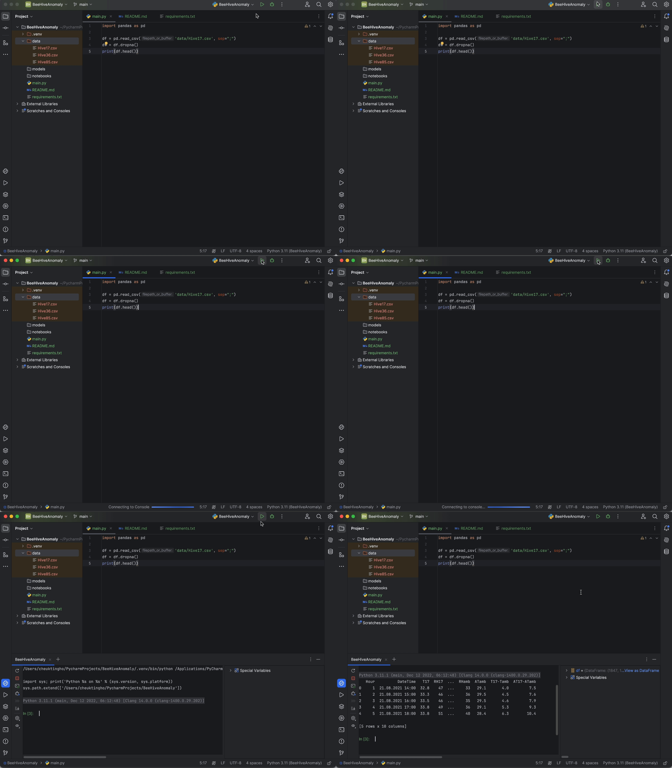
4. Fit the data points and inspect them in a graph
Since we’ll be using the OneClassSVM from scikit-learn, we’ll import it together with DecisionBoundaryDisplay and Matplotlib using the code below:
from sklearn.svm import OneClassSVM
from sklearn.inspection import DecisionBoundaryDisplay

import matplotlib.pyplot as plt
According to the data’s description, we know that column T17 represents the temperature of the hive, and RH17 represents the relative humidity of the hive. We’ll extract the value of these two columns as our input:
X = df[["T17", "RH17"]].values
Then, we’ll create and fit the model. Note that we’ll try the default setting first:
estimator = OneClassSVM().fit(X)
Next, we’ll show the decision boundary together with the data points:
disp = DecisionBoundaryDisplay.from_estimator(
    estimator,
    X,
    response_method="decision_function",
    plot_method="contour",
    xlabel="Temperature", ylabel="Humidity",
    levels=[0],
)
disp.ax_.scatter(X[:, 0], X[:, 1])
plt.show()
Now, save and press Run again, and you’ll see that the plot is shown in a separate window for inspection.
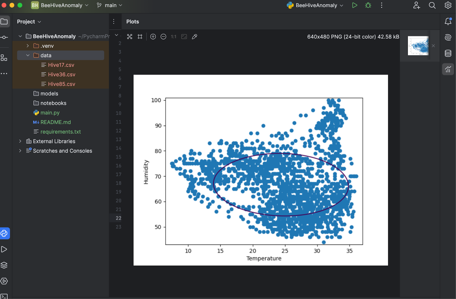
5. Fine-tune hyperparameters
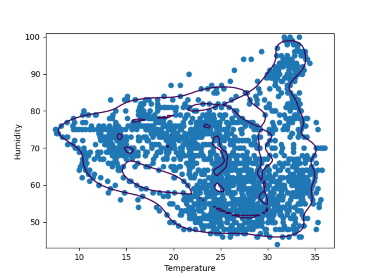
As the plot above shows, the decision boundary does not fit very well with the data points. The data points consist of a couple of irregular shapes instead of an oval. To fine-tune our model, we have to provide a specific value of “nu” and “gamma” to the OneClassSVM model. You can try it out yourself, but after a couple of tests, it seems “nu=0.1, gamma=0.05” gives the best result.
Example: Isolation Forest
Isolation Forest is an ensemble-based method, similar to the more popular Random Forest classification method. By randomly selecting parting features and values, it will create many decision trees, and the path length from the root of the tree to the node making that decision will then be averaged over all the trees (hence “forest”). A short average path length indicates anomalies.

Now, let’s compare the result of OneClassSVM with IsolationForest. To do that, we’ll make two plots of the decision boundaries made by the two algorithms. In the following steps, we’ll build on the script above using the same hive 17 data.
1. Import IsolationForest
IsolationForest can be imported from the ensemble categories in Scikit-learn:
from sklearn.ensemble import IsolationForest
2. Refactor and add a new estimator
Since now we’ll have two different estimators, let’s put them in a list:
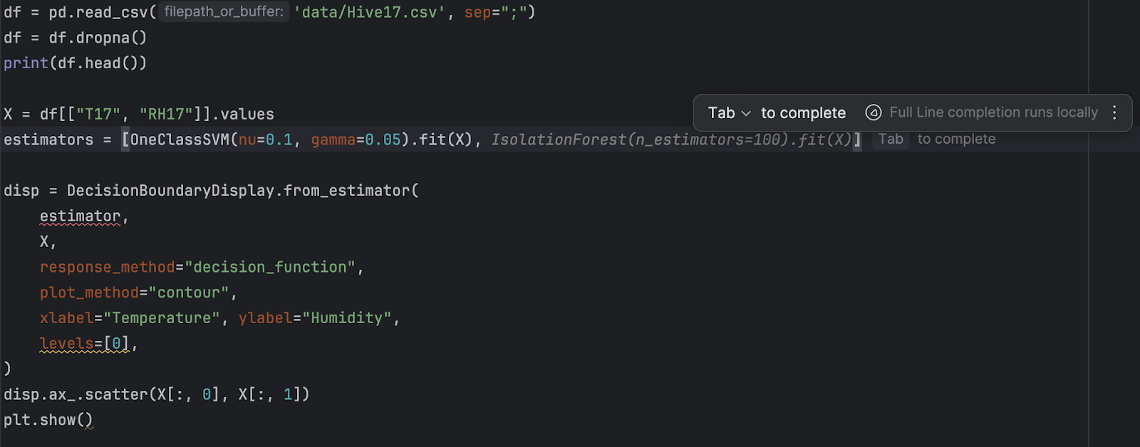
estimators = [
    OneClassSVM(nu=0.1, gamma=0.05).fit(X),
    IsolationForest(n_estimators=100).fit(X)
]
After that, we’ll use a for loop to loop through all the estimators.
for estimator in estimators:
    disp = DecisionBoundaryDisplay.from_estimator(
        estimator,
        X,
        response_method="decision_function",
        plot_method="contour",
        xlabel="Temperature", ylabel="Humidity",
        levels=[0],
    )
    disp.ax_.scatter(X[:, 0], X[:, 1])
    plt.show()
As a final touch, we’ll also add a title to each of the graphs for easier inspection. To do that, we’ll add the following after disp.ax_.scatter:
disp.ax_.set_title(
        f"Decision boundary using {estimator.__class__.__name__}"
    )
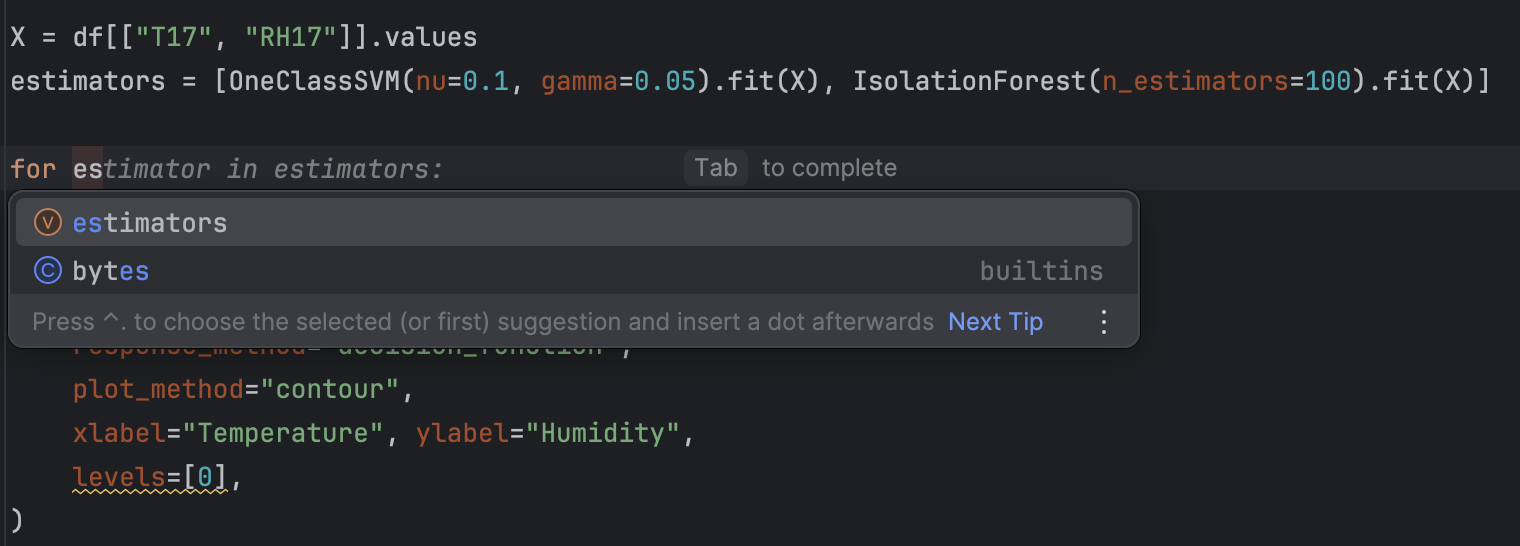
You may find that refactoring using PyCharm is very easy with the auto-complete suggestions it provides.
3. Run the code
Like before, running the code is as easy as pressing the Run button in the top-right corner. After running the code this time, we should get two graphs.
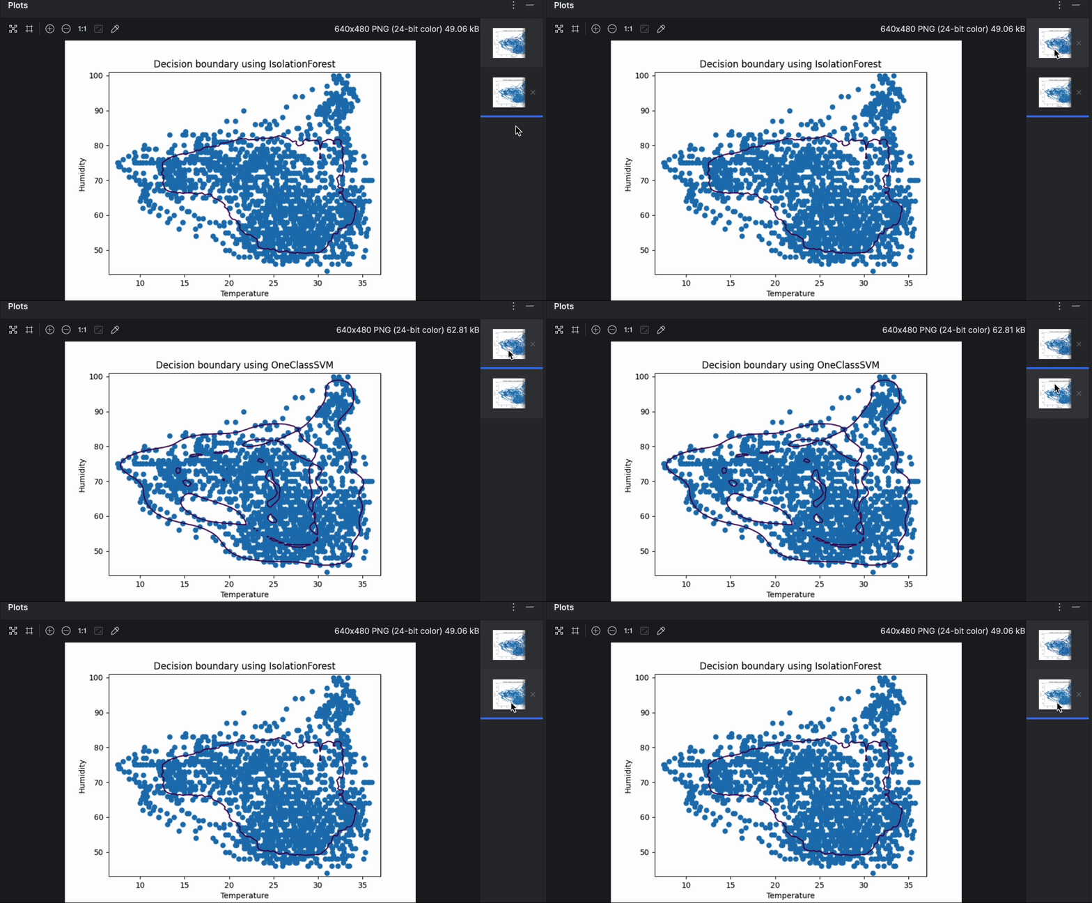
You can easily flip through the two graphs with the preview on the right. As you can see, the decision boundary is quite different while using different algorithms. When doing anomaly detection, it’s worth experimenting with various algorithms and parameters to find the one that suits the use case the most.
Next step: anomaly detection in time series data
If the data is like our bee hive data, which is a time series, then there are additional methods to single out anomalies. As time series have trends and periods, anything out of this pattern of trends and periods can be considered as anomalies. Popular methods to detect anomalies in time series include STL decomposition and LSTM prediction.
Learn how to use these methods to detect anomalies in time series in this blog post.
Summary
Anomaly Detection has proven to be an important aspect of business intelligence, and being able to identify anomalies and prompt immediate actions to be taken is essential in some sectors of business. Using the proper machine learning model to automatically detect anomalies can help analyze complicated and high volumes of data in a short period of time. In this blog post, we have demonstrated how to identify anomalies using statistical models like OneClassSVM.
To learn more about using PyCharm for machine learning, please check out “Start Studying Machine Learning With PyCharm” and “How to Use Jupyter Notebooks in PyCharm”, “Jupyter-native Python IDE for ML”.
Detect anomalies using PyCharm
With the Jupyter project in PyCharm Professional, you can organize your anomaly detection project with a lot of data files and notebooks easily. Graphs output can be generated to inspect anomalies and plots are very accessible in PyCharm. Other features, such as auto-complete suggestions, make navigating all the Scikit-learn models and Matplotlib plot settings a blast.
Power up your data science project by using PyCharm; check out the Databricks-integrated data-science IDE offered to streamline your data science workflow.


