Quantitative Research in Python: Using Notebooks
This is a first in a series of blog posts covering the use of Python for quantitative research. In this post, we take a look at IPython Notebooks: a really handy tool for structuring calculations in a document-like fashion.
If you look at the state of various computer algebra systems (CASs) today, you will see that they typically operate not only on the basis of a REPL-style console window input, but rather provide a workbook/worksheet/document mechanic whereas the commands to be executed and their results are mixed together. This effectively provides for literate programming and makes it easy to write entire articles/books directly from a CAS.
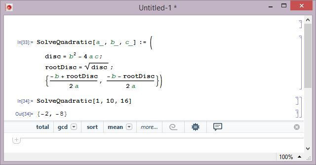
Python is no exception: it has taken the world of numerical computing by storm, becoming a serious contender to established programming languages such as MATLAB or R. And indeed, the exact mode of interaction is supported in Python too with the use of IPython Notebooks.
The IPython Notebook
First of all, make sure you’ve actually got Python and IPython. The simpliest way of doing this is to simply install a distribution package that includes lots of pre-built Python tools, such as Contunuum’s Anaconda or Enthought Canopy.
The IPython Notebook support is part of the IPython distribution. Its goal is to provide a web-based document editing experience whereas the user can enter one of two things:
- Ordinary text (Markdown format) that will be presented as such. Among other things, IPython Notebooks support LaTeX formatting, which is great for rendering formulae.
- Python code, which is stored in cells. You can execute each of the cells and the output will appear right after the relevant cell.
Here’s what typical interaction with a workbook looks like:
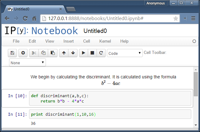
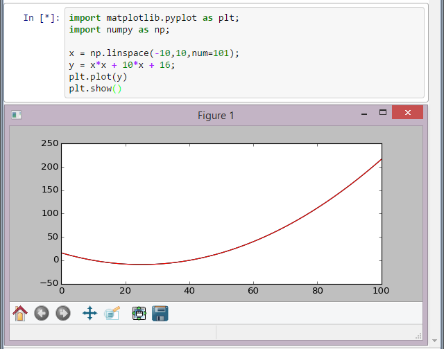
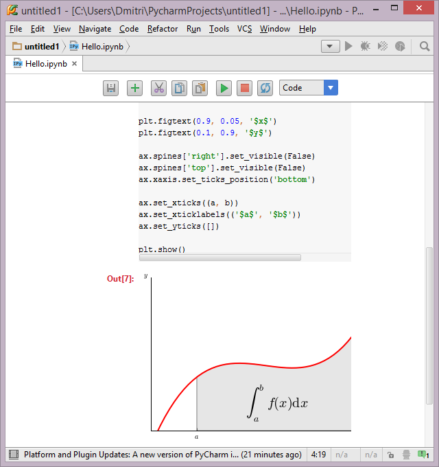
Now, you could be forgiven for thinking that this form of interaction only supports textual output. In actual fact, it supports graphical output too, so you can do data visualizations with libraries such as Matplotlib. Simply import the package and call its APIs and you’ll get the visual output right here on the page:
While the IPython notebooks are great when used on the web, they offer little help when coding. Sure, they report on the errors in your cells, but apart from non-automatic code completion, they do not offer any coding assistance features (e.g., automatic code completion, parameter info, navigation, as-you-type error checking, and so on), so you essentially need to know the API by heart and rely on the interpreter itself to catch your errors. Alternatively, you can just use PyCharm.
Notebooks in PyCharm
Using IPython notebooks in PyCharm is easy, and gives you the benefit of PyCharm’s features such as code completion. Here’s how to do it.
Note: an active IPython notebooks instance is only required for evaluation of Python code. Text rendering is handled by PyCharm itself.
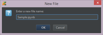
First, create a file with an .ipynb extension. This signals to PyCharm that it’s an IPython notebook.
Second, makes sure an IPython Notebook kernel is running. The simplest way is to simply fire up PyCharm and when you try to evaluate something, you will see the following dialog:
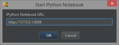
Simply enter the URL and PyCharm will fire up an IPython notebook at this exact location.
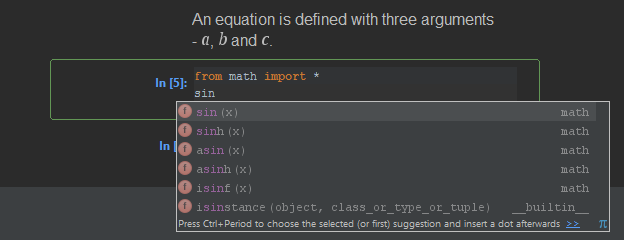
Finally, go ahead and edit the cells in the document. Unlike the web interface, PyCharm provides a lot of things: you get code completion, inspections and navigation features that you would expect if you were working with an ordinary Python project:
Press Ctrl+Enter to execute a cell. Note that the cell number gets incremented accordingly. Press Shift+Enter to add a new cell.
If you want to add some text or a heading, use the drop-down menu to pick the appropriate element. Text entries also support LaTeX — use a single $ to delimit inline formulae and two dollars ($$) for display formulae.
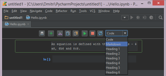
Finally, it’s worth noting that PyCharm’s theming is matched in the worksheet, so if you prefer a more article-like feel, this is possible too:
Libraries for Quantitative Analysis
The simplest kinds of libraries that you need for quantitative analysis are mathematical libraries such as NumPy and SciPy. These packages contain a wealth of different numerical method implementations.
When it comes to visualization, there is the excellent matplotlib library that we already mentioned.
And of course there are plenty of wrappers around native libraries available to Python through the power of tools like SWIG. For example, the QuantLib library uses it to generate Python wrappers around its C++ interfaces. It’s not an ideal process, but it does produce a workable package that you can use.
Naturally, Python also has other bindings which might be useful when analyzing and visualizing data. These include things such as tools for building interactive applications (e.g., wxPython) or bindings to NVIDIA CUDA via PyCuda.
So, that’s it for now! Enjoy IPython notebooks!

