PyCharm Scientific Mode with Code Cells

You can use code cells to divide a Python script into chunks that you can individually execute, maintaining the state between them. This means you can re-run only the part of the script you’re developing right now, without having to wait for reloading your data. Code cells were added to PyCharm 2018.1 Professional Edition’s scientific mode.
To try this out, let’s have a look at the raw data from the Python Developer Survey 2017 that was jointly conducted by JetBrains and the Python Software Foundation.
To start, let’s create a scientific project. After opening PyCharm Professional Edition (Scientific mode is not available in the Community Edition), choose to create a new project, and then select ‘Scientific’ as the project type:
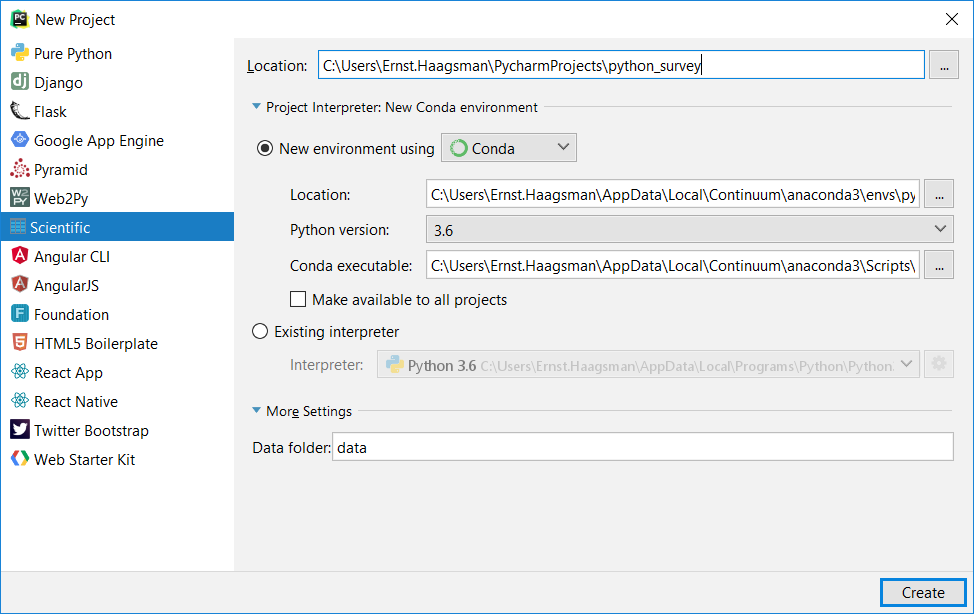
A scientific project will by default be created with a new Conda environment. Of course, for this to work you need to have Anaconda installed on your computer. The scientific project also creates a folder structure for your data.
If we want to analyze data, we’ll first need to go get some data. Please download the CSV file from the ‘Raw Data’ section of the developer survey results page. Afterward, place it in the `data` folder that was created in the scientific project’s scaffold.
Extract, Transform, Load
Our first challenge will be to load the file. The easiest way to do this would be to run:
import pandas as pd
pd.read_csv(‘data/survey.csv’)
So let’s run this. After writing this code in the `main.py` file that was created for us with the project, right click anywhere in the file and choose ‘Run’. We should see a Python console appear at the bottom of our screen after the script completes execution. On the right-hand side, we should see the variable overview with our dataframe. Click ‘View as DataFrame’ to inspect the DataFrame:
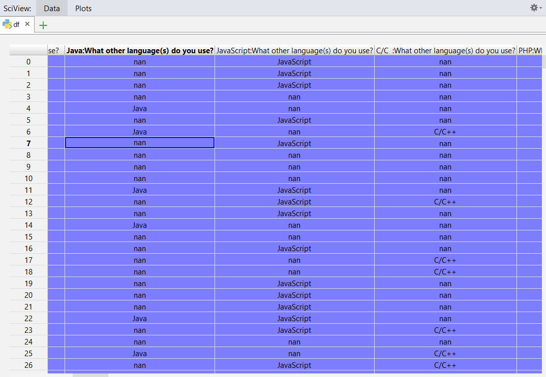
We can see the structure of the CSV file here. The columns have headings like “Java:What other language(s) do you use?”. These columns are the result of multiple-choice answers: respondents were asked ‘What other language(s) do you use?’ and could select multiple answers. If an answer was selected, that string is inserted. Otherwise the string ‘NA’ is inserted (if you open the CSV file directly, you’ll be able to see a lot of ‘NA’ values).
If you scroll through the DataFrame a little more, you’ll see that in some cases Pandas was able to correctly infer some data, but in many cases it would be fairly unwieldy to work with the data in this shape.
To make the data easier to work with, we could recode columns after the read_csv call, and fix things. A better way is to configure the `read_csv` call with various parameters.
In this step, we’d like to make sure that our columns will be named in a way that’s easier to work with, and to make sure that the data types are all correct. To do this, we can use several parameters of `read_csv`:
- names – allows us to specify the names of the columns (instead of reading them from the CSV file). We need to pay attention to the fact that if we specify this parameter, Pandas will import the header column as a data row by default. We can prevent that by explicitly specifying `header=0`, which indicates that the 0th row (the first row) is a header row.
- dtype – enables us to specify a datatype per column, as a dict. Pandas will cast values in these columns to the specified datatype.
- converters – functions that receive the raw value of the cell for a specified column, and return the desired value (with the desired datatype).
- usecols – allows us to specify exactly which columns to import.
For more details, see the documentation for read_csv. Or, just write `pd.read_csv` in PyCharm to see it in the documentation tool window (this works if you have scientific mode enabled; if not, use Ctrl+Q to see the documentation).
The disadvantage of these parameters is that they take lists and dicts, which become very unwieldy for datasets with many columns. As our dataset has over 150 columns, it would be a pain to write them inline. Also, the information for one column would be spread among these parameters, making it hard to see what is being done to a column.
One great thing about analyzing data with Pandas is that we can use all features of the Python language. So let’s create a data dictionary with plain Python objects, and then use some Python magic to transform these to the structures Pandas needs.
The Data Dictionary
To recap, for every column we want to know what name we will want to give it, and how to encode the values. We also want to have the ability to drop a column.
Let’s create a separate file to hold our data dictionary: `survey_data_dictionary.py`. In this file, we define a class that describes what we want to do with a column:
class ColumnDescription:
   def __init__(self, full_name, name='', dtype=None, converter=None, usecol=True):
       self.full_name = full_name
       if name:
           self.name = name
       else:
           self.name = full_name
       self.dtype = dtype
       self.converter = converter
       if self.dtype is not None and self.converter is not None:
           raise ValueError("Define either a dtype or a converter, not both")
       self.usecol = usecol
Now we can make a big list of all of our columns, and describe one-by-one what to do with them. To make our lives easier, we can use Pandas to get a list of the current names of the columns. Run in the Python console:
for col in df.columns:
    print(‘#{}’.format(col))
This will print the full name of every column as a Python comment. Copy & paste the full list into the data dictionary Python file after the class definition. We can now use regex replacement to create instances of our `ColumnDescription` class.
Open the Replace tool (Ctrl+R or Edit | Find | Replace), and make sure to check ‘Regex’ to enable regex mode. Enter `#([^\n]+)` as the regex to find. This looks for the ‘#’ character, and then multiple characters that are *not* a newline. Everything between the parentheses is captured into a group, which we can then use in the replacement (use $1 for the first capture group).
As a replacement type (use Ctrl+Shift+Enter to create newlines):
ColumnDescription(
    full_name=”$1”
),
Make sure you’ve indented the middle line, and used double quotes, and then click “Replace all”. Now we’ve created a lot of `ColumnDescription` objects. We’ll need them in a list for Pandas, so let’s wrap it with a list constructor now. Write `DATA_DICTIONARY = [` before the first `ColumnDescription` call, and `]` at the end of the file. Choose Code | Reformat Code to properly indent all of the `ColumnDescription` calls.
At this point, we can go back to our `main.py` and feed this data structure into the `read_csv` call. Let’s start by adding the ability to rename columns – we do this with the `names` parameter. This should be a list of strings, with as its length the number of columns in the CSV file.
We can use a Python list comprehension to extract the names from our list of `ColumnDescription` objects:
from survey_data_dictionary import DATA_DICTIONARY

names = [x.name for x in DATA_DICTIONARY]
At this point we can provide this list to `read_csv`. We also need to remember to specify the header row explicitly so that Pandas doesn’t import the header row as a data row:
df = pd.read_csv(‘data/survey.csv’, names=names, header=0)
If we run this code, we should see nothing has changed. To see if it worked, let’s go back to our data dictionary and add a name to the first column:
ColumnDescription(
   full_name="Is Python the main language you use for your current projects?",
   name="python_main"
),
After re-running main.py, we should now see that the first column has been renamed. Crack open a bottle of champagne to celebrate your success!
Let’s provide the other metadata from DATA_DICTIONARY to `read_csv` with a combination of list comprehensions and dict comprehensions:
# Generate the list of names to import
usecols = [x.name for x in DATA_DICTIONARY if x.usecol]

# dtypes should be a dict of 'col_name' : dtype
dtypes = {x.name: x.dtype for x in DATA_DICTIONARY if x.dtype}

# same for converters
converters = {x.name: x.converter for x in DATA_DICTIONARY if x.converter}

df = pd.read_csv('data/survey.csv',
                header=0,
                names=names,
                dtype=dtypes,
                converters=converters,
                usecols=usecols)
Now all that’s left to do is to populate the rest of the data dictionary. Unfortunately, this is manual work; there’s no way for Pandas to know the design of our survey. If you want to follow along with the rest of the blog post without writing the entire data dictionary, you can grab a complete one from the GitHub repo.
For those columns that are either ‘NA’ or the name of the selected columns, we can create a small helper function that will convert these to booleans:
def notNA(text):
	return text != ‘NA’
We can then specify this helper function as the converter for a column like this:
ColumnDescription(
   full_name="Java:What other language(s) do you use?",
   name="otherlang_java",
   converter=notNA
),
Another type of data that’s fairly common in surveys is categorical data: multiple choice, single answer. We can specify Pandas’ CategoricalDType as the data type for those columns:
ColumnDescription(
   full_name="What do you think is the ratio of these two numbers?:Please think about the total number of Python Web Developers in the world and the total number of Data Scientists using Python.",
   name="webdev_science_ratio_self",
   dtype=CategoricalDtype(
       ["10:1", "5:1", "2:1", "1:1", "1:2", "1:5", "1:10"],
       ordered=True
   )
),
Cleaning up our Data
Although our columns are now looking good, we may want to make some additional changes to our data. In the Python developer survey, the first question was:
Is Python the main language you use for your current projects?
- Yes
- No, I use Python as a secondary language
- No, I don’t use Python for my current projects
All respondents who selected they don’t use Python were excluded from most of the rest of the survey. So we should drop these data points for our analysis. Let’s create a new code cell, and start cleaning up our data.
Code cells are defined simply by creating a comment that starts with `#%%`. The rest of the comment is the header of the cell, which you see when you collapse it:
#%% Cleaning the data
As long as you have the scientific mode enabled in PyCharm Professional, you should see a dividing line appear, and a green ‘play’ icon to run the cell.
It’s fairly easy to select data in Pandas, so let’s complete our cell:
#%% Cleaning the data

df = df[df['python_main'] != "No, I don’t use Python for my current projects"]
As the remaining choices are basically “Yes” and “No”, we can also turn the remaining data into a boolean:
df[‘python_main’] = df[‘python_main’] == ‘Yes’
Analyzing our Data
In our survey, users were asked what they thought the ratio is between the number of Python developers creating web applications, and the number of developers that do data science. To make things interesting, they were also asked what they thought other people thought this ratio was. Let’s see now if people think they agree with the rest of the world.
The questions look like this:
Please think about the total number of Python Web Developers in the world and the total number of Data Scientists using Python.
What do you think is the ratio of these two numbers?
Python Web Developers ( ) 10:1 ( ) 5:1 ( ) 2:1 ( ) 1:1 ( ) 1:2 ( ) 1:5 ( ) 1:10 Python data scientists
What do you think would be the most popular opinion?
Python Web Developers ( ) 10:1 ( ) 5:1 ( ) 2:1 ( ) 1:1 ( ) 1:2 ( ) 1:5 ( ) 1:10 Python data scientists
Make sure you’ve specified categorical data types in the data dictionary for both questions.
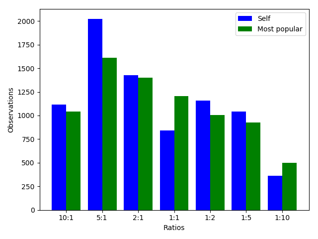
We can now go ahead and create a new code cell to start our analysis. Let’s start by getting the value counts:
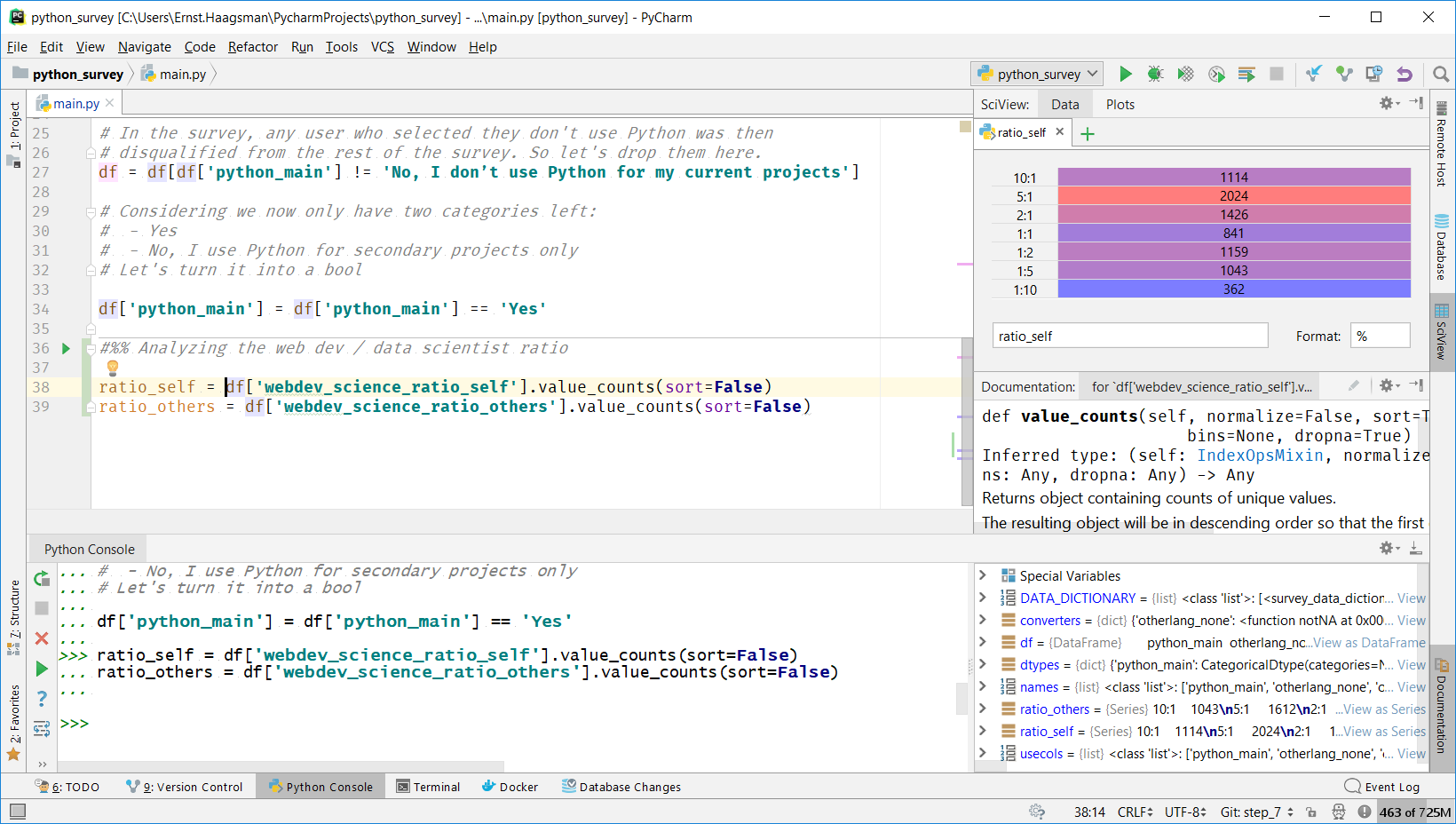
ratio_self = df['webdev_science_ratio_self'].value_counts(sort=False)
ratio_others = df['webdev_science_ratio_others'].value_counts(sort=False)
We’re disabling sorting here to maintain the order that we’ve specified using the categorical data type. If we run this cell with the green play icon, we can then click ‘View as Series’ in the variable overview to have a glance at our data.
We can also use Matplotlib to get a graphical overview of the data:
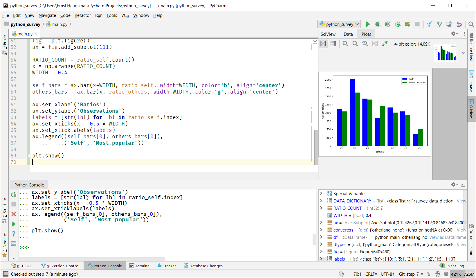
See the GitHub repository for the exact code used to generate the plot.
We can see in the plot that there’s a difference between what individual respondents thought the ratio was, and what they thought the most popular opinion was. So let’s dive a little deeper: how big is this difference?
Exploring Further
Although the data points are categorical, they represent numbers, so we can see what the numeric difference would be if we turn them into numbers. Let’s create a new code cell, and calculate the difference:
CONVERSION = {
   '10:1': 10,
   '5:1' : 5,
   '2:1' : 2,
   '1:1' : 1,
   '1:2' : 0.5,
   '1:5' : 0.2,
   '1:10': 0.1
}

self_numeric = df['webdev_science_ratio_self'] \
                   .replace(CONVERSION.keys(), CONVERSION.values())

others_numeric = df['webdev_science_ratio_others'] \
                   .replace(CONVERSION.keys(), CONVERSION.values())

print(f'Self:\t\t{self_numeric.mean().round(2)} web devs / scientist')
print(f'Others:\t\t{others_numeric.mean().round(2)} web devs / scientist')
After running this cell, we see:
Self:       3.23 web devs / scientist
Others:     3.02 web devs / scientist
Turns out the difference in means isn’t very large. However, the distributions are fairly different. We can see in the plot that the ‘self’ distribution has a peak at the 5:1 web dev:data scientist point, whereas the ‘Most popular’ distribution trades some votes from 5:1 to 1:1. Fun fact: this same survey found about a 1:1 distribution between web developers and data scientists with its Python usage questions.
To see whether or not we have a significant difference, we can use a Chi-Square test. The scipy.stats package contains a method to calculate this statistic. So let’s create a last code cell to finish this investigation:
#%% Is the difference statistically significant?

result = scipy.stats.chisquare(ratio_self, ratio_others)

# The null hypothesis is that they're the same. Let's see if we can reject it

print(result)
This results in: `Power_divergenceResult(statistic=294.72519972505006, pvalue=1.1037599850410103e-60)`.
In other words, there’s a 1-60 chance that this is the result of random chance, and we can conclude this is a statistically significant difference.
What’s Next?
We’ve just shown how to ingest a fairly large CSV file into Pandas, and how to handle the conversion of data from its raw form to a form that’s easier to analyze. For the example, we looked into what respondents think the Python ecosystem looks like. And we’ve confirmed that people think that others have a different opinion from themselves (also, water is wet).
Now it’s your turn! Download the CSV (and you may want to grab the data dictionary from this blog post’s repo) and let us know what interesting things you discover in the Python developer survey! It contains many interesting data points: what people use Python for, what their job roles are, what packages they use, and more.