The Story of AI Graphics at JetBrains


Generating art at JetBrains
At JetBrains, we are constantly refining our approach to creating pieces of art for use as website elements and release graphics. Our mission is to free graphic designers from routine tasks so they can concentrate on their core competence – creativity. The history of internal tools for generating art at JetBrains starts about a decade ago. At first, we mainly used WebGL-based tools, which generated everything randomly in the browser on the fly (the interactive archive is available here). The images below were created with this approach.

Splash screens that were created using WebGL.
In 2020, we released our first tool based on deep neural networks. Since then, everything has been generated in a K8s GPU cluster using PyCharm and Datalore for local and remote development. The browser is used only for input-output. With this approach based on neural networks, we’ve achieved a much higher degree of personalization, allowing us to cater to our designers’ needs, and we are constantly working to improve it.
These pictures were made with a compositional pattern-producing network (CPPN, top) and Stable Diffusion (SD, bottom). This post will cover the technical details of both approaches, as well as the way we combine them to create even more spectacular designs.

Splash screens that were generated with neural networks.
CPPNs: An overview
CPPNs are among the simplest generative networks. They simply map pixel coordinates (x, y) to image colors (r, g, b). CPPNs are usually trained on specific images or sets of images. However, we found that randomly initialized CPPNs produce beautiful abstract patterns when the initialization is done correctly).

CPPN architecture: pixel coordinates are inputs, RGB values are outputs.
Using the usage data from an early internal version of the generator, we refined our algorithms to improve the visual quality. Aside from that, we also slightly extended the classical architecture of CPPNs by introducing multiple virtual parameters. Hence, our CPPNs now map (x, y, a, b, c, f) to (r, g, b). This simple change allows us to introduce an easy-to-use, although somewhat unpredictable, method for altering the image, as shown below.
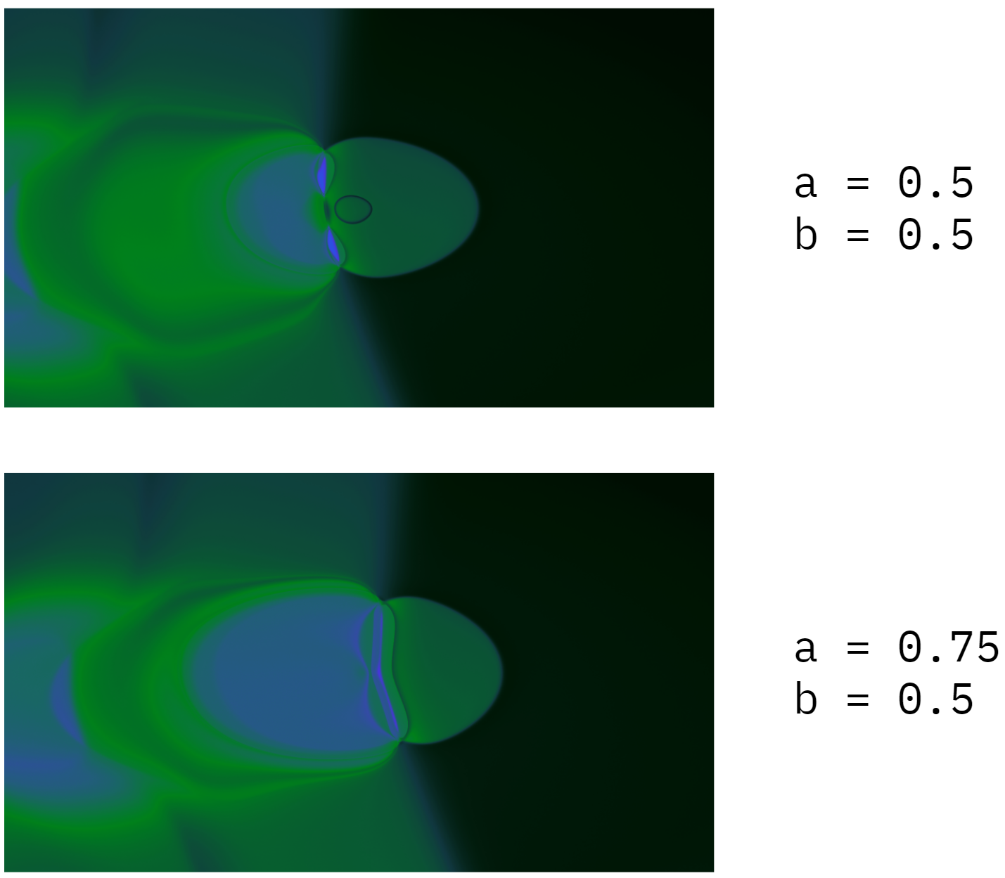
By updating the virtual parameter (a), we’re slightly changing the picture.
These virtual parameters don’t have to be constant. For example, we can map the value of the virtual parameter f of each pixel to the distance from this pixel to the center of the image. This trick allows us to ensure the image has circular shapes. Or we could map f to the sum of the absolute values of the pixel’s coordinates, which will yield diamond-shaped patterns. This is where math actually meets art!
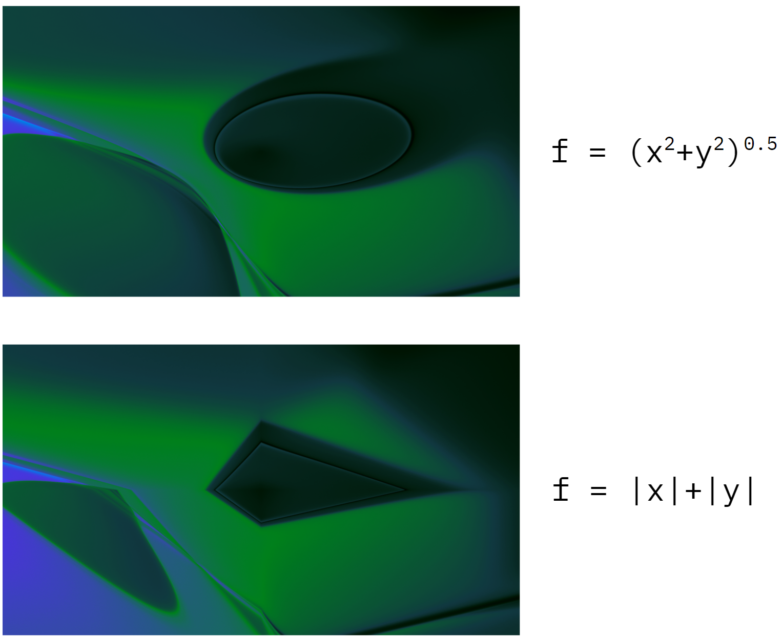
Different functions f(x,y) result in different image patterns.
To ensure that our randomly initialized CPPNs always produce beautiful designs, we trained a recommendation system to predict whether the given set of parameters will result in an image that looks good. We trained our algorithm from user feedback received during internal testing. The figure below shows two examples of images created by randomly initialized CPPNs and their corresponding “beautifulness” scores.
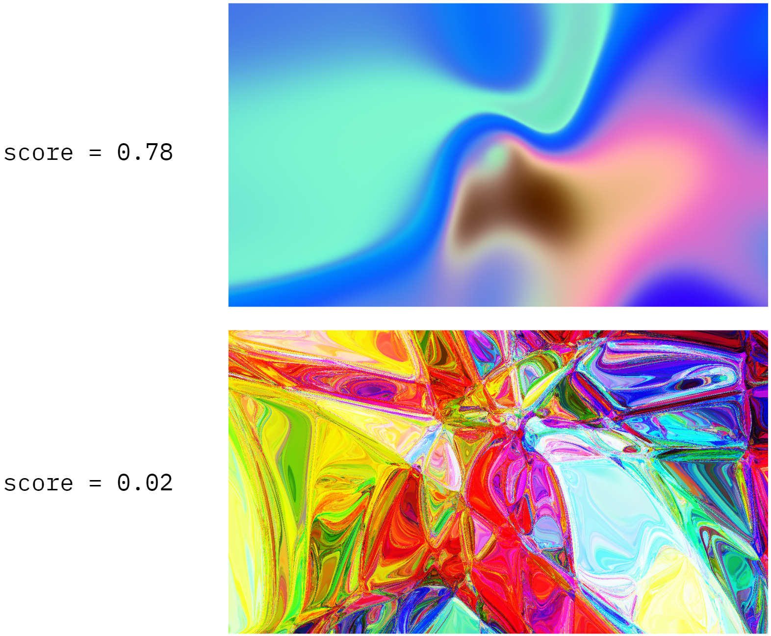
Predicting “beautifulness” scores of CPPN images.
CPPNs: Animation
Our CPPN-generated works of art really come to life when they are transformed into video graphics. By mapping virtual parameters (a, b, c) over any closed parametric curve (one that starts and ends at the same point), we can create seamlessly looped animations of any desired length!
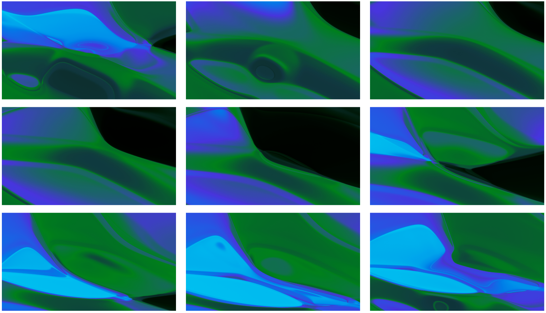
Sample frames of a CPPN animation video.
The choice of a curve function is crucial. Animating virtual parameters over a plain circle is the most straightforward approach. However, it has a drawback: when the sign of a parameter changes (for example, from 0.01 to -0.01) while it has a low first derivative value (one that equals zero in the case of a circle trajectory), the result is usually a shaky animation. To account for this issue, we use Bernoulli’s lemniscate to ensure that the signs of the virtual parameters never change (see the image below). This solves the shaky animation problem, but introduces a new one. For most animation frames, one of the parameters is only incrementally updated, making the animation look too shallow. We addressed this by switching to a random spline function. The more complex the trajectories we used, the richer the animation looked!
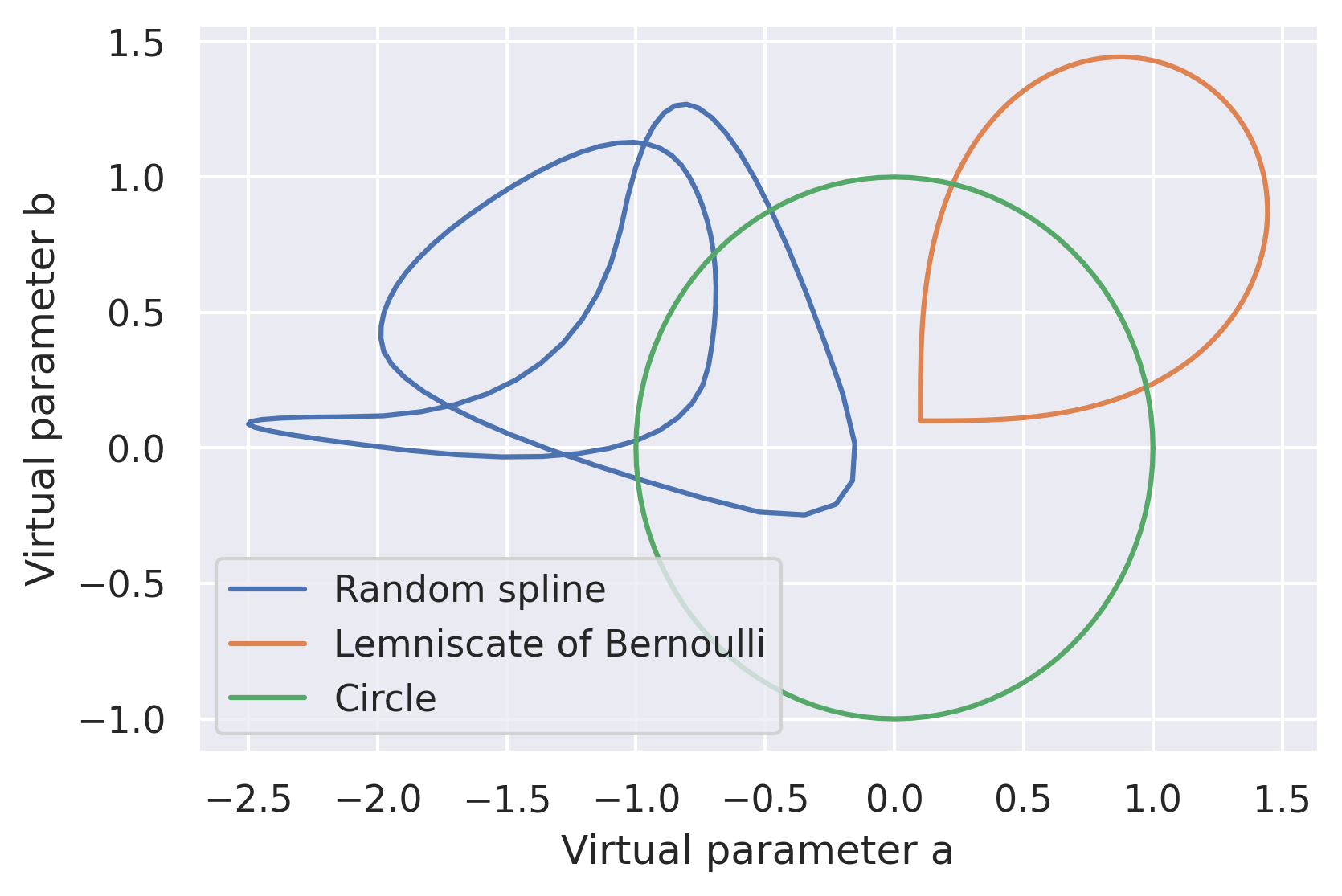
Examples of CPPN curve functions.
CPPNs: Color correction
There’s one more crucial detail: color correction. Our CPPNs – and therefore the resulting images – are randomly generated, but we need to ensure that each uses our brand colors. We tried a few different approaches to achieve this. The first iteration (used in the 2020 releases) relied on SVG recoloring directly in the browser (using feColorMatrix and feComponentTransfer). This approach was quick – since the recoloring happened in the browser, we could update the palette without re-rendering the image on the server side. However, it was tricky to implement as some palettes are too complex for feColorMatrix and feComponentTransfer and it was generally unreliable. After extensive experimentation, we found that the resulting colors could differ depending on the browser and the operating system. Here is an example from our experiments in early 2020. On the left is a screenshot of a background of the earlier generator version made on a setup using Safari on macOS, and on the right is a screenshot of the same background but from a setup using Google Chrome on Ubuntu Linux. Notice the subtle brightness discrepancies. The more post-processing effects we applied, the more prominent they became.
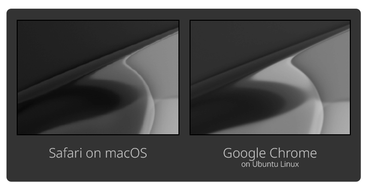
An example of brightness discrepancies.
Another example is MDN’s sample of feComponentTransfer. This time, both images were made on the same machine using Ubuntu Linux and Google Chrome, but on the left image, hardware acceleration was disabled. There are prominent color discrepancies, especially between the Table lookup examples. Thus, despite being very quick, this approach to color correction was extremely inconsistent.
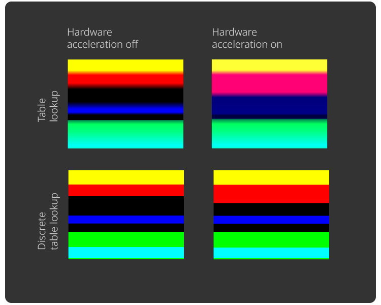
An example of color discrepancies.
Our current approach (in use since 2021) is more straightforward. We render source images in 32-bit grayscale, meaning that instead of RGB, our CPPNs return only a single luminance value. We then map each pixel to a lookup table with precomputed ideal RGB values. This approach is slower but produces pixel-perfect results.
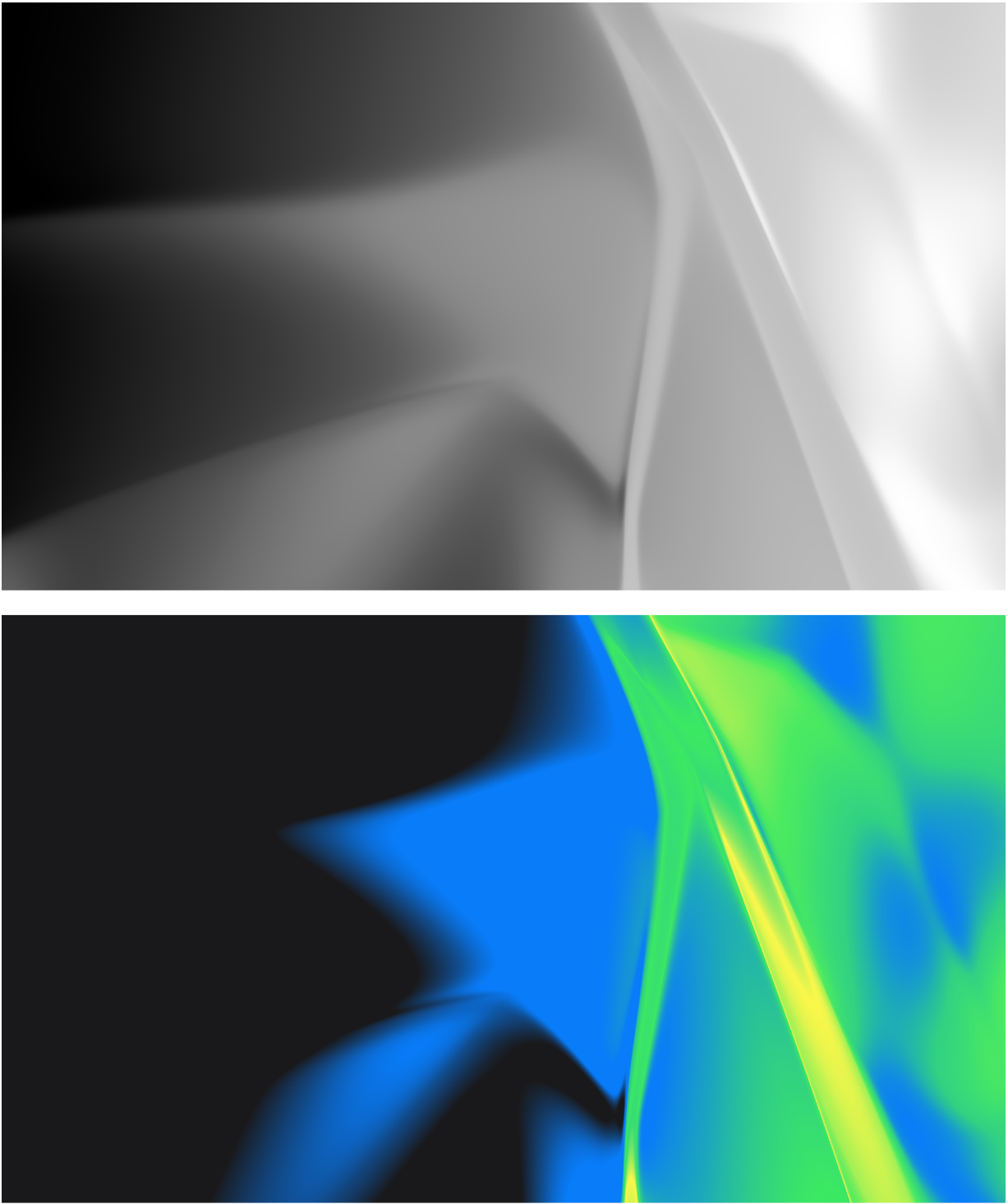
An example of color correction using a grayscale image.
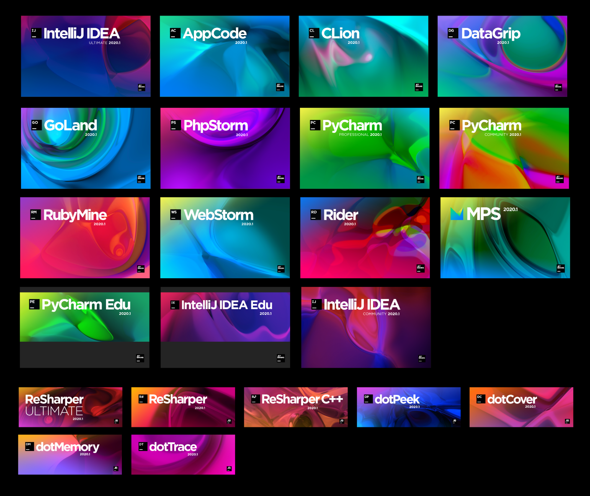
2020.1 splash screens that used SVG recoloring.
When our current approach to color correction is used alongside the CPPN with virtual parameters and spline animation, the result is a video like this!
Another remarkable property of CPPNs is that, due to their simple architecture, it’s very easy to translate their computational graphs to GLSL code. Once the animation video is ready, we can export it as a WebGL fragment shader and then directly run it in the browser. An example of the results of this approach is Qodana’s landing page.
Our CPPN-based generator is available here.
To dive deeper into CPPNs, check out our public Datalore notebook with code examples:
Taming Stable Diffusion
Stable Diffusion offers a high level of versatility and visual fidelity, making it a perfect backbone for our art generators. To make Stable Diffusion appropriate for use as a source of release graphics, we had to adhere to the following criteria:
- Images should follow the brand palette.
- No artifacts or glitches (such as broken pixels) are allowed.
- It should be easy to use a specific style (abstract smooth lines) out of the box.
- It should require little to no prompting, meaning it should provide accessible and intuitive controls.
Though there is always room for improvement, we’ve met all of these requirements. The latest images are publicly available, and all of the technical details are below.
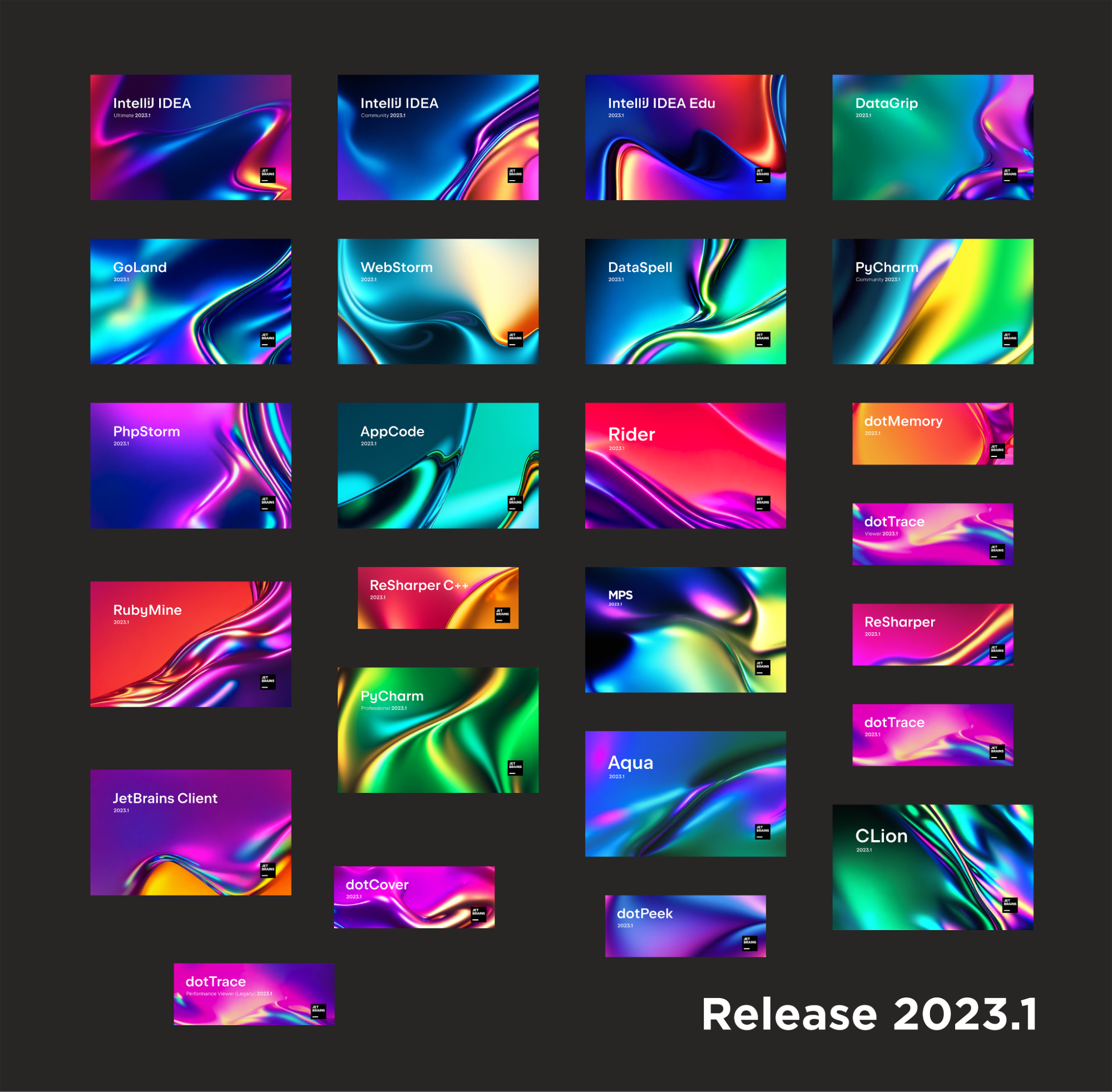
2023.1 splash screens created with Stable Diffusion.
To produce results that consistently met all of our criteria, we fine-tuned Stable Diffusion using various references provided by our designers. Below are some examples of images generated according to various styles.
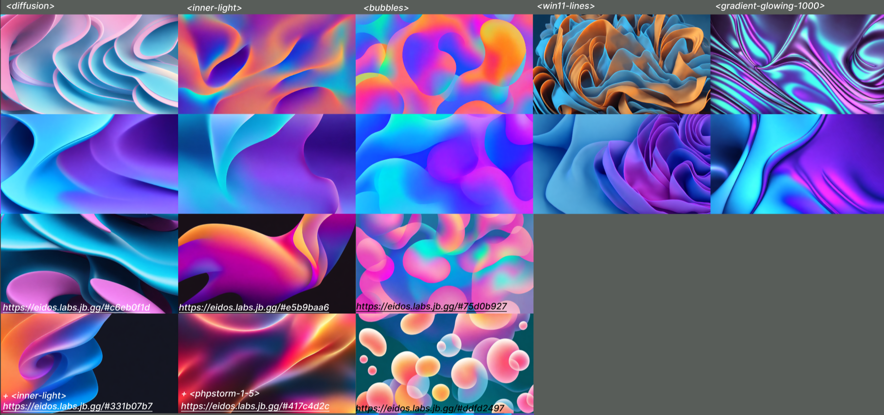
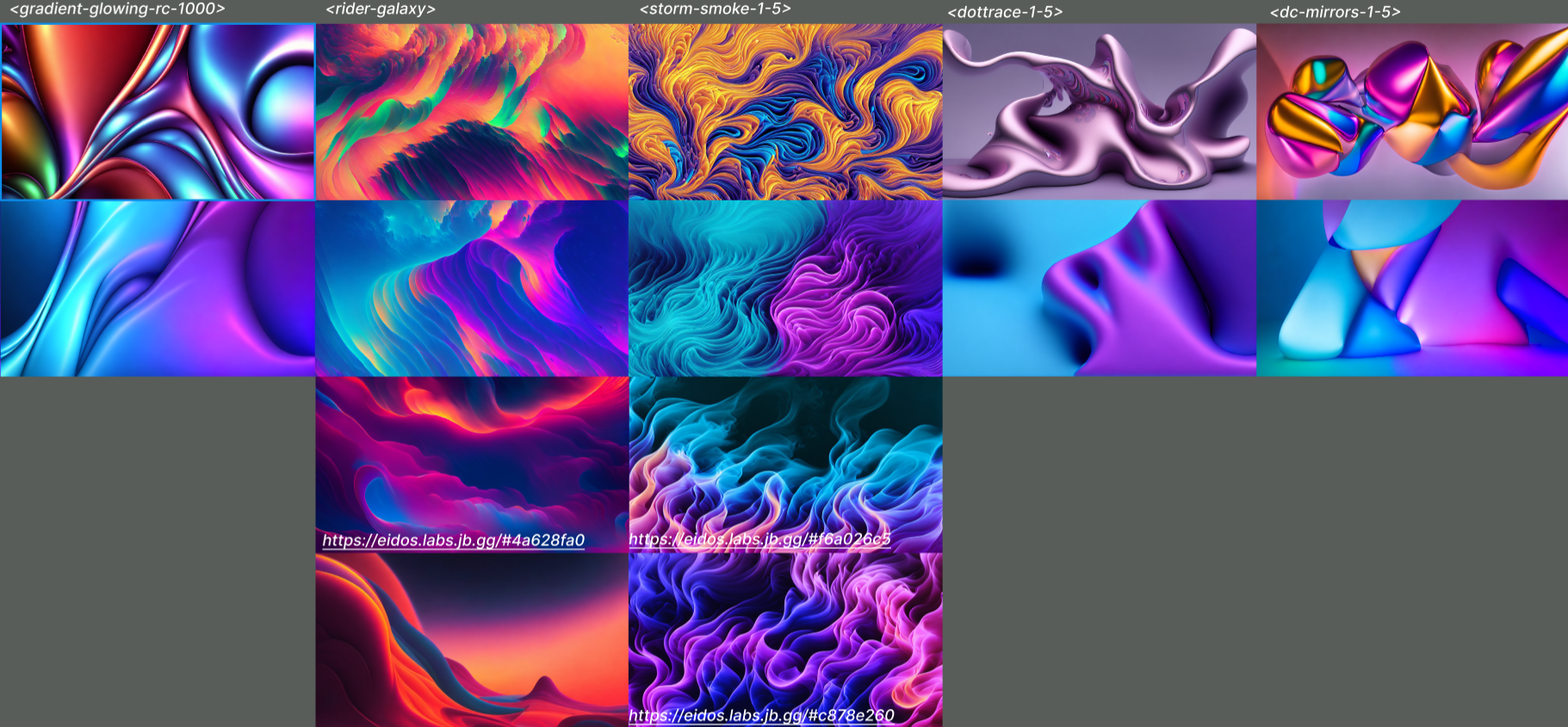
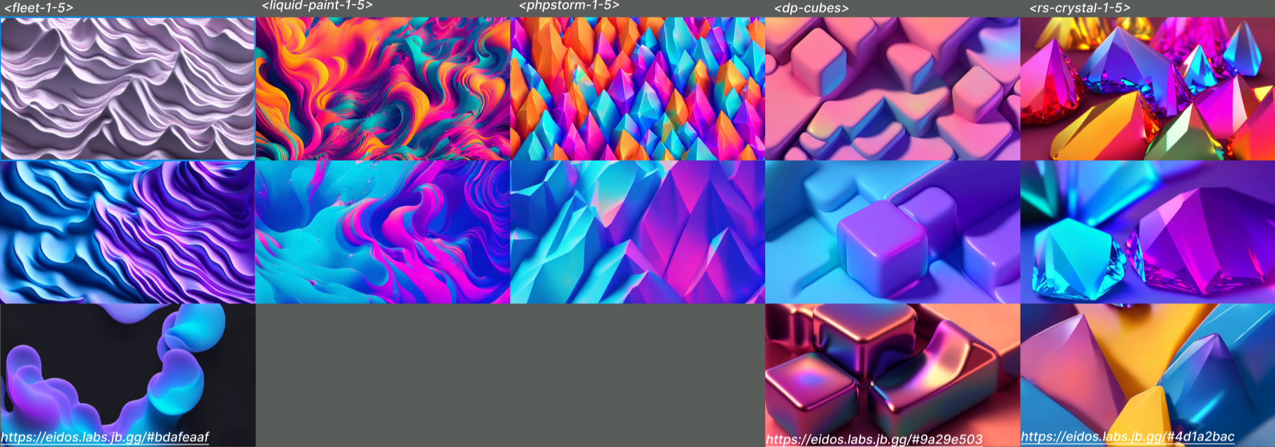
Experimental styles obtained by fine-tuning Stable Diffusion.
Before diving into the technical details of the fine-tuning process, let’s look at the internals of Stable Diffusion. It essentially consists of three parts: the CLIP text encoder (a tiny transformer model used for encoding text into a multi-modal embedding space), a variational autoencoder that compresses and decompresses images to and from latent space, and the denoising UNet.
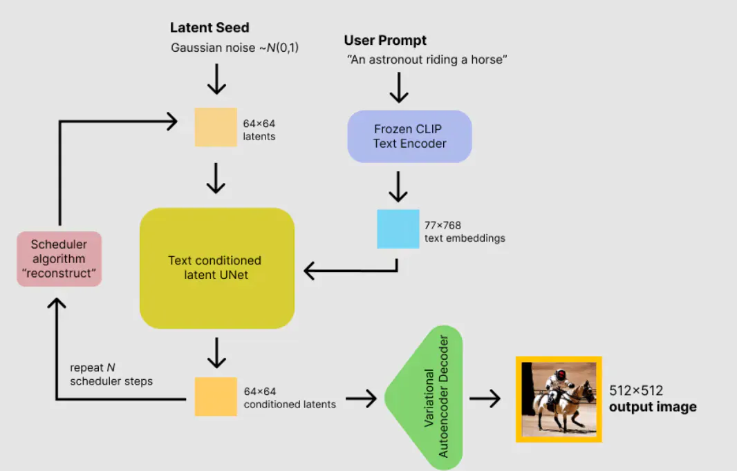
The architecture of Stable Diffusion. Image source: www.philschmid.de/stable-diffusion-inference-endpoints.
The generation process is roughly as follows:
- We encode the prompt text into an embedding, which is a 77×768 floating-point array.
- We randomly generate the latent representation of the image, which could be either pure Gaussian noise or a noised representation of an init image.
- We repeatedly pass the encoded latent image and encoded text through the denoising UNet for a given number of steps.
- After denoising the latent image, we pass it through the decoder, thus decompressing it into a standard RGB image.
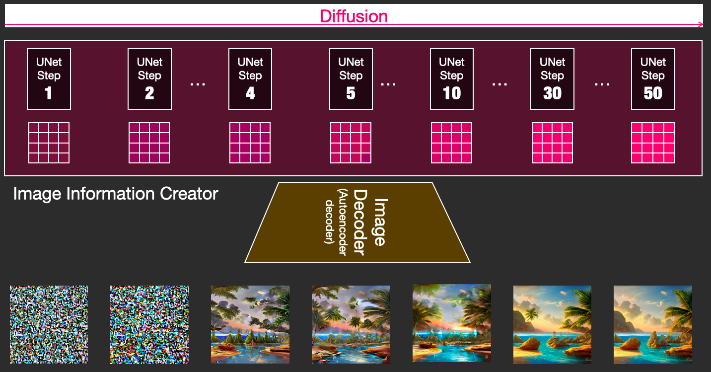
The denoising process. Image source: jalammar.github.io/illustrated-stable-diffusion/.
Crucially for us, the great thing about Stable Diffusion is that it’s possible to fine-tune it with very little data and achieve great results! As a side effect, data-efficient fine-tuning methods are also computing-efficient, which makes it even better.
The most straightforward fine-tuning approach is textual inversion (p-tuning). We freeze all of the weights, such as UNet, VAE, and the text encoder (meaning we don’t update them during training), and only train one new word per embedding for the text encoder. Because we only train one new word per embedding, there are only 768 trainable parameters!
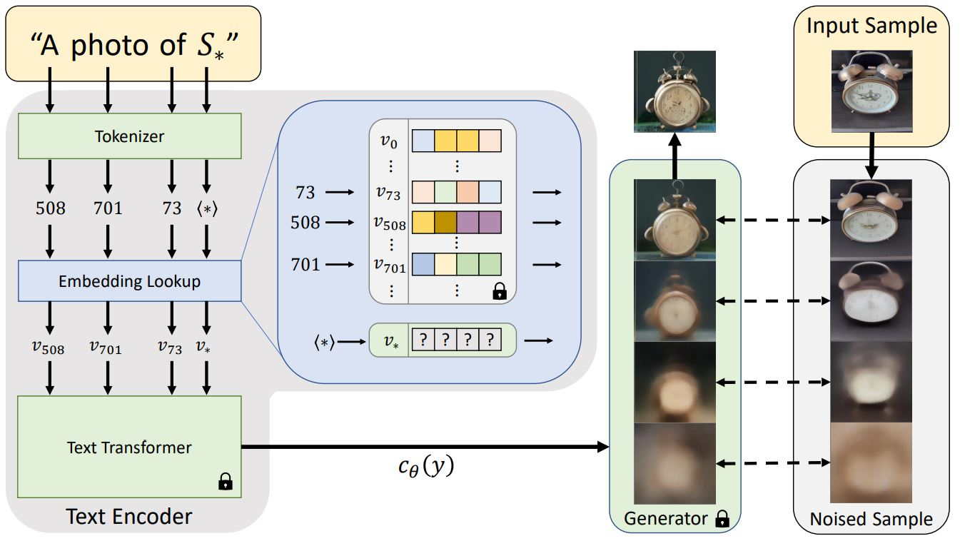
Outline of the text-embedding and inversion process. Image source: textual-inversion.github.io/.
These custom embeddings are composable, meaning we could use up to 77 embeddings in a single prompt. On top of that, they are easy to train, taking ~2 hours on a single RTX 4090. Below is an example of the training process. Both of these images were generated using the prompt “digital art in the style of <sculpture>”, where “<sculpture>” is the new word embedding that we’re training. As we perform more training steps, the image evolves, and the new visual style becomes more and more pronounced.
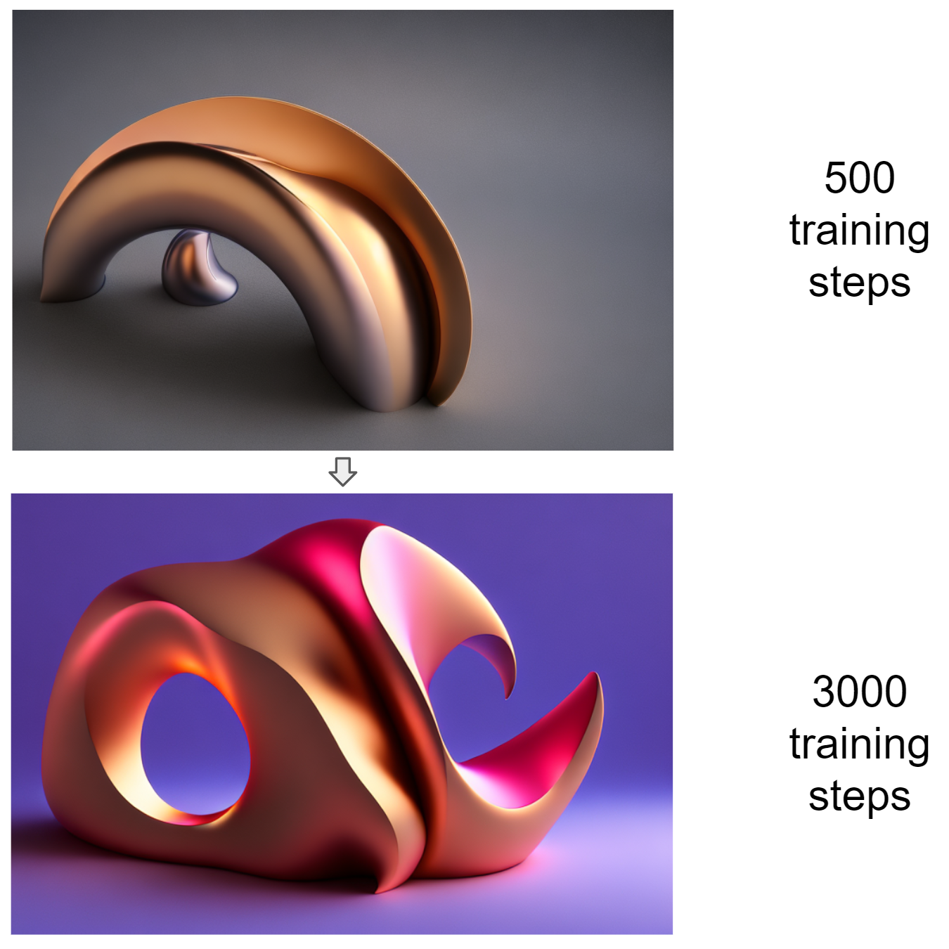
The image generated with the textual inversion after 500 and 3000 training steps.
Another popular and efficient fine-tuning method is Low-Rank Adaptation, or simply LoRA. The key idea of LoRA is similar to textual inversion, only this time in addition to freezing the weights we also introduce new ones by adding small adapter layers to attention layers inside UNet.
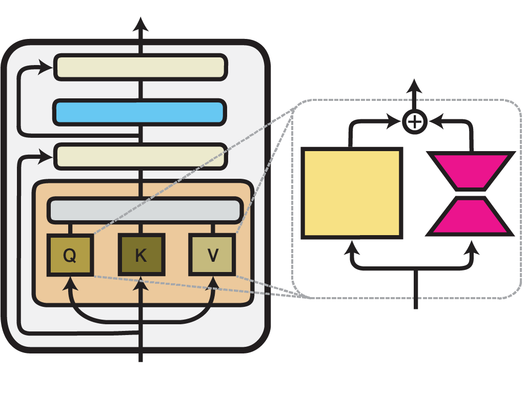
Illustration of the LoRA method within one Transformer layer. Image source: adapterhub.ml/blog/2022/09/updates-in-adapter-transformers-v3-1/.
Compared to textual inversion, this approach makes it possible to capture more sophisticated patterns from the fine-tuning data (for example, “AI portrait” apps work by training adapter layers on the user’s face), but it uses slightly more resources and, most importantly, multiple LoRAs cannot be composed. In our specific use case, we found that LoRA is most effective when working with Stable Diffusion XL. By contrast, in earlier versions of Stable Diffusion (1.4, 1.5, or 2.1), textual inversion allows for more versatility.
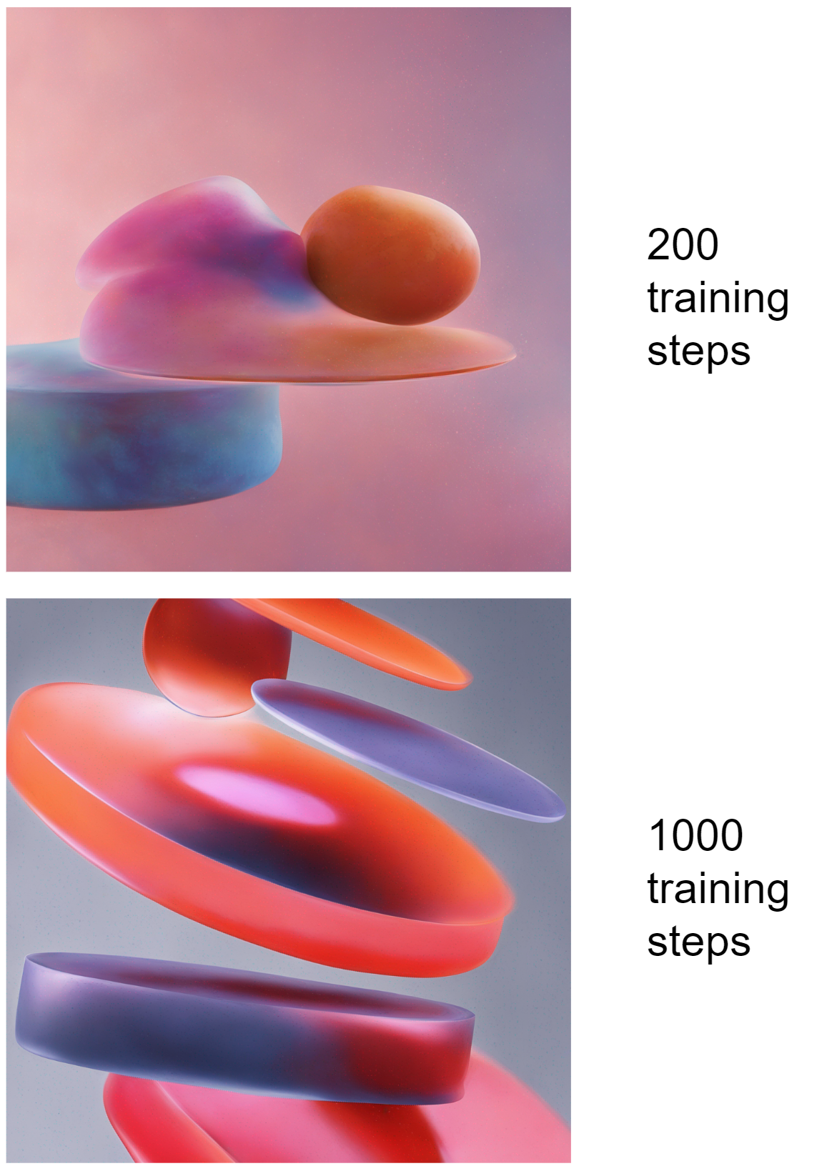
The image generated with LoRA after 200 and 1000 training steps.
Combining the strengths of Stable Diffusion and CPPNs
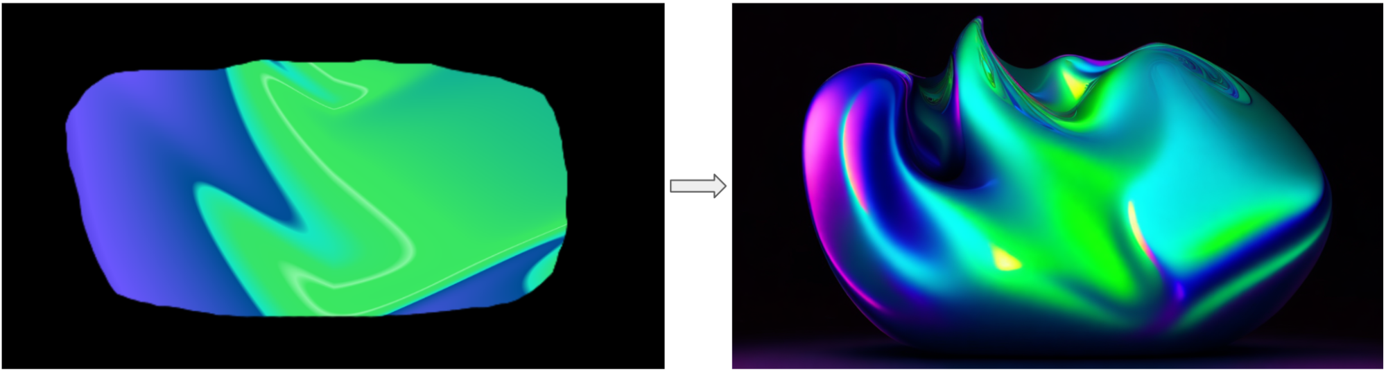
One of our criteria for using Stable Diffusion was the need to ensure that the generated images follow the color palette of some particular brand, and this is where CPPNs come to our aid! Before generating an image with Stable Diffusion, we generate an image with CPPN using our Gradient generator (described above), apply the desired colors with pixel-perfect accuracy, then encode it with VAE and mix it with Gaussian noise. UNet uses the resulting latent image as its starting point, thus preserving the original colors and composition.


CPPN → Stable Diffusion pipeline.
Once the CPPN image is ready, we can also edit it directly in the browser to achieve any shape and design we could ever imagine!
CPPN → Stable Diffusion pipeline with manually edited CPPN image.
Finally, once we have produced multiple images with our “CPPN → Stable Diffusion” pipeline, we can train another CPPN on those images and turn them into an animation, as described in the CPPNs: Animation section above! Here’s some example GLSL code, along with some example videos:
The exploration and implementation of AI-powered graphics at JetBrains has been an adventure. Our tools have evolved and matured over the years, from our initial approach using WebGL-based random generation to our current use of CPPNs and Stable Diffusion to generate sleek and personalized designs. Moving forward, we anticipate greater levels of customization and versatility, and we are excited about the possibilities these technologies will unlock in the graphics generation field.
We hope this in-depth look into our AI art journey has been illuminating! We invite you to explore the examples we’ve provided (including our interactive archive) and share your feedback here in the comments or via cai@jetbrains.com. Please let us know what kinds of topics you would like to see from the Computational Arts team in the future!